Week 12 - Validation studies of Symmetry BC vs Wedge BC in OpenFOAM vs Analytical H.P equation

Laminar pipe flow in OpenFOAM using symmetry and wedge BC:

In last exercise, the pipe flow was simulated using wedge BC on a pipe sector with `2^0` wedge section, 11.55 [m] length and 0.01 [m] diameter. The same pipe dimensions are used for this exercise as well with varying sector angles of `10^0, 25^0 and 45^0`.The domain will be solved using both wedge and symmetry boundary conditions on faces at sector ends.

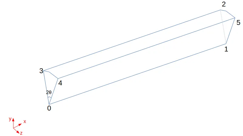
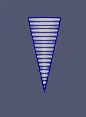
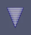
Same nomenclature as in previous section is used to describe the domain for blockMeshDict files. The blockMeshDict files are generated using the matlab utility created in previous exercise by changing the wedge angle and patch type. Wedge boundary condition solves the domain in 2D with axissymmetric assumption. Symmetry boundary condition solves the domain in 3D with zero gradient applied on symmetry faces. Hence 1 cell is used z direction for wedge boundary condition case. The cases using symmetry boundary condition can have multiple cells in z direction to resolve the difference in `theta` direction. However using multiple cells in `theta` direction will result in very skewed cells near the axis, where long thin prisms will be formed. This will lead to solution difficulties. To maintain the solution stability `10^0` case is solved with 1 cell layer; `25^0` case is solved with 2 cell layers and `45^0` case is solved with 4 cell layers in z direction. For symmetry BC cases, the number of cells in z direction are manually changed in blockMeshDict files. The test folder, "pipe" generated in previous exercise is copied to 6 folders for each sector angle of different BC types and renamed appropriately. Mesh files are generated using blockMesh command in the test folders with updated blockMeshDict files placed in system folder.

BC \Angle	`10^0`	`25^0`	`45^0`
Wedge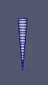
Symmetry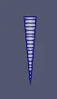

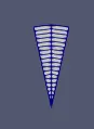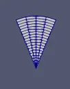Initial conditions and solver settings are retained from preivous exercise. Solution is solved for 100 seconds, to complete approximately 2 flow-throughs with time-step value of 0.1 [s]. Solution is processed through icoFoam solver and the flow reaches steady state in all the 6 cases.

Results comparison:

1. Hydrodynamic-length:

Hydrodynamic entry length is the length of pipe required for the flow to reach fully developed flow profile, where the velocity profiles and wall shear stress become constant along the pipe length. Here the wall shear stress along the pipe wall is plotted for all the cases with wedge and symmetry boundary conditions. Almost all the cases have same wall-shear-stress profile except `25^0` and `45^0` wedge cases.

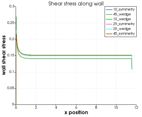
Hydrodynamic length as deduced from the plot above is 1.8 [m] where the wall shear stress reaches constant value. `25^0` and `45^0` wedge cases have slighly smaller entry lengths.`45^0` case is showing a large variation in wall shear stress values in fully developed section of pipe compared to other cases.

2. Velocity profile

Velocity profile in cross-section of pipe becomes constant along the length of pipe in fully developed flow region. Velocity profile at the diamter of outlet is plotted againt y-coordinate for all the cases. Analytical solution for velocity profile is also calculated and plotted in the same graph.

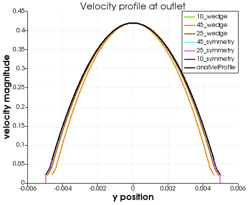
Almost all the cases have velocity profile matching with the analytical solution - shown in black, except for 2 cases - `25^0` and `45^0` wedge BC. `45^0` wedge case shows the highest deviation from analytical solution.

3. Max velocity and pressure drop

Maximum velocity is seen on the axis of the pipe flow where the shear stress is relatively minimum. Velocity magnitude is plotted against x-coordinate along the axis of the pipe length for all the cases.

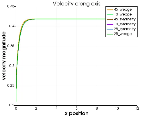
From the plot, all cases seem to converge on a value of 0.42 [m/s] at axis in fully developed flow region. This is twice the average velocity value of 0.21 [m/s] specified as inlet velocity. Hence, the analytical solution of maximum velocity in pipe flow is met by all the cases. `25^0` and `45^0` wedge cases seem to reach maximum velocity slightly earlier than other cases, suggesting shorter entry length. This corresponds to our observation using wall shear stress.

Pressure drop is calculated by getting the average kinematic pressure at inlet using integrate variables option in paraView and multiplying it by density of the fluid flowing in the domain. Since, outlet BC is specified with 0 kinematic pressure, average inlet kinematic pressure corresponds to the kinematic pressure drop in the pipe. Pressure drop as calculated from Hagen-Poiseuille's equation in previous exercise came to a value of 776.16 [Pa]. This is used to calculate the percentage deviation of pressure drop for each case against the analytical solution.

	avg inlet pessure x 10^3 [Pa]	pessure drop [Pa]	error-`Deltap` %
`10^0` wedge	0.809232	809.232	4.26
`25^0` wedge	0.841412	841.412	8.4
`45^0` wedge	0.936353	936.353	20.63
`10^0` symmetry	0.809187	809.187	4.25
`25^0` symmetry	0.812556	812.556	4.68
`45^0` symmetry	0.81077	810.77	4.45

Minor difference in pressure drop is expected as the entry length is not neglected in the calculation. All cases except `25^0` and `45^0` wedge cases show around 4% difference in pressure drop which is acceptable. However, the `25^0` case shows 8% difference while `45^0` case shows much larger deviation of around 20%.

4. Shear stress

Shear stress values as obtained in paraFoam are plotted against y-lines in fully developed flow region for all the cases.

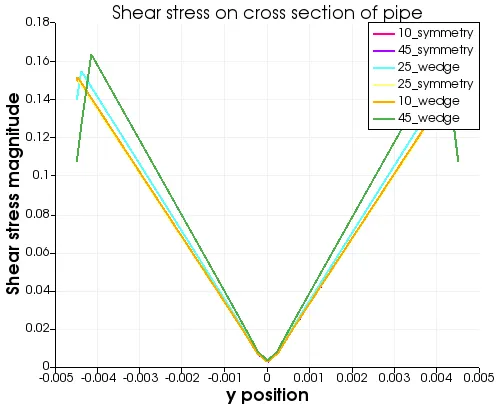
Similar to previous observations, `25^0` and `45^0` wedge cases deviate in shear stress profiles compared to other cases. All other cases have matching shear stress profiles in cross-section of pipe. The shape of the shear stress profiles are as expected in analyitcal solution except for the near wall region. This is due to the divergence method used in paraView to calculate shear stress and can be ignored.

5. Wedge vs symmetry boundary conditions

Wedge boundary condition requires a single cell layer between the wedge faces. The domain is solved in 2D with axisymmetric assumption. The wedge boundary condition works great with smaller wedge angles - less than `5^0`, for axissymmetric flow problems such as uniform laminar pipe flow. The computational effort is greatly reduced by solving the problem in 2D on reduced number of cells. Also the axissymetric nature of the flow is maintained. However, this boundary fails to reproduce analytical or correct solution when the wedge angle is large, such as `25^0 and45^0` cases used above.

Symmetry boundary condition is used when the flow behavior is symmetric across a plane. The plane can be assumed as symmetry boundary and only half of the domain can be used for solving the problem. This boundary condition can be used in both 2D and 3D problems, which can considerably reduce the computational effort. The cases using symmetry boundary condition with different sector angles produced almost identical results confirming the flow behavior is axisymmetric. With sufficient number of cells to resolve the flow gradients, any value of `theta` can be used to represent the domain with symmetry boundary condition for such flows. However opting for wedge boundary condition in such scenarios is more prudent since reduced computational effort is required for domains using wedge boundary condition. Symmetry boundaries are useful when the flow is not axissymmetric but the flow gradient are negligible across a sector plane such as the midplane.