Week 12 - Final Project - Modelling and Analysis of a Datacenter
Aim: To model a data center using Macros and do a thermal simulation to understand the airflow patterns and temperature stratification within the data center space.
Objectives:
- To create the data center components using Macros.
- To mesh the model with appropriate assumptions.
- To set up the physics model to get the solution
- To interpret the results using different types of plots and animation.
Creation of the data centers components like computer room air conditioning units (CRACs), server cabinets, power distribution units (PDUs), and perforated floor tiles
First of all, on opening the ICEPAK project is named Data_Center_Analysis.
Since this is a big project Macros are to be used. All dimensions and data are given in imperial units so, from the Edit menu preference tab is selected to change the units to imperial units, default dimensions to Start/Length, numerical display precision to 2, lineWidth to 2 for blocks, fans, openings, plates,
resistances, and grilles, for this project only.
Now the Creation of Data Center Components
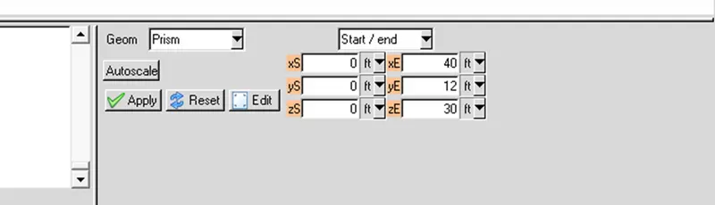
Resizing of default cabinet to the given dimensions.
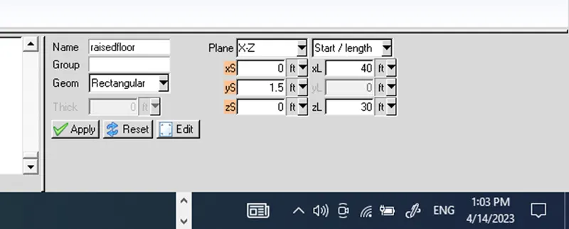
Creation of Raised Floor
By clicking on create plate command and modifying dimensions as given in the problem.
Creation of the first CRAC unit
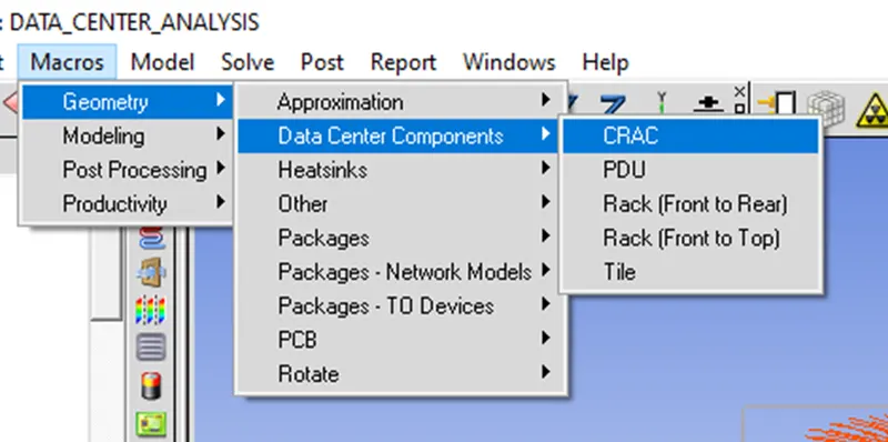
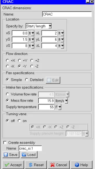
Once we select CRAC from the Macros, we will get a template as given below, then the data fields are populated with the given data of CRACs in the problem.
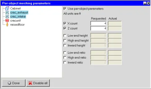
From the mesh control local tab Per-object Meshing Parameters for the Fans are modified as given below:
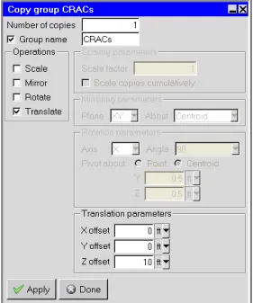
A new group named CRACs for the CRAC unit is created by selecting crac_unit and then crac_exhaust in the Model Manager window.
The second CRAC unit is created by copying group CRACs entities and translating them in the z-direction by 10 fits.
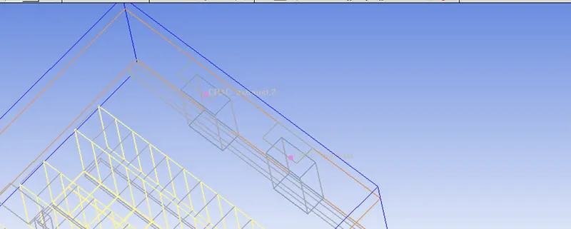
CRACs as placed in the cabinet shown below:
Creation of a row of server racks
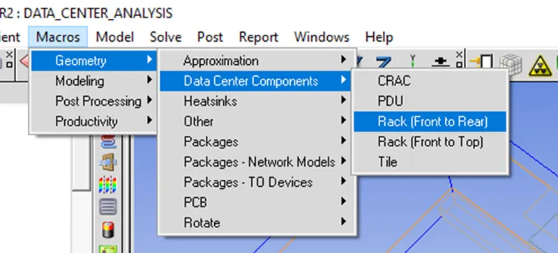
After selecting Rack (Front to Rear) from Macros, data fields are populated in the template as shown below:
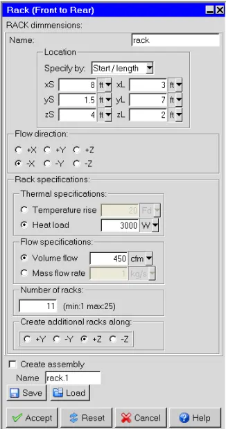
Creating a new group for the server racks by selecting rack and then rack-opens. 10 in the Model Manager window is done.
A second row of server racks is created by copying group RACKs as shown below:
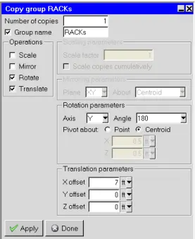
Creating a row of high-density server racks.
Dimensions and flow, and power data are filled as given below:
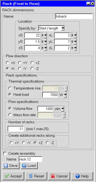
Creating a new group for the high-density server racks by selecting hdrack and then hdrack-opns.10
in the Model Manager window and Named it as HDRACKs.
Create a second row of high-density server racks.
Created a second row of high-density server racks by copying HDRACKs in the Groups node by selecting Rotate and Translate in the Operations group box as Axis to Y and the Angle to 180 and X offset to 7 ft.
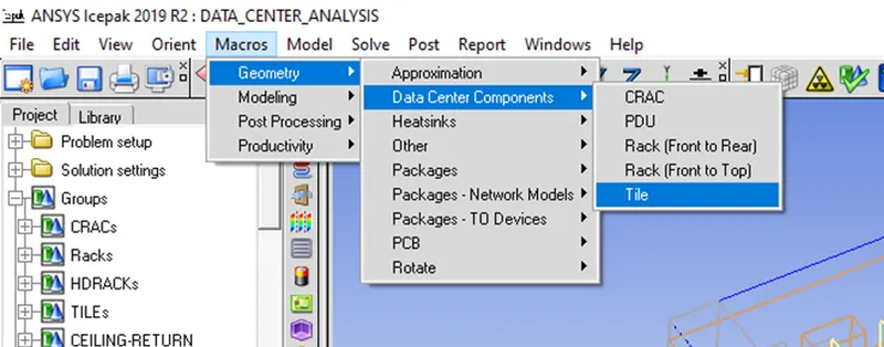
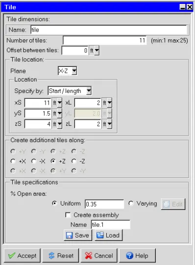
Create a row of perforated tiles.
The steps followed are shown below and data fields are populated by the given data.
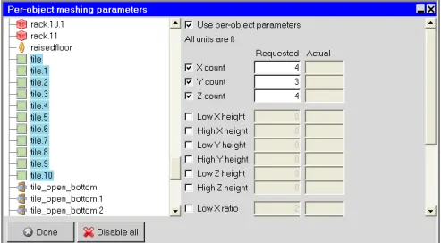
Per-object meshing parameters are set from the local tab of mesh control as shown below:
Created a new group for the perforated tiles by selecting tile and then tile_open_bottom.10 in the Model
Manager window and named as TILEs.
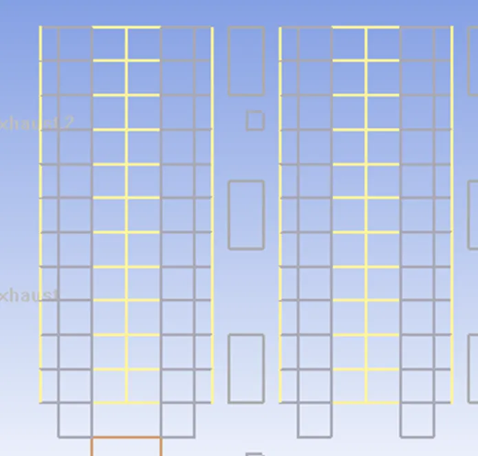
Created three more rows of perforated tiles by copying TILEs in the Groups node and by selecting translate and X offset to 2 ft. Copied TILEs in the Groups node again and set Translate and the X offset to 14 ft to create another row of tiles.
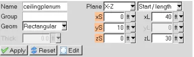
Created the ceiling plenum by selecting create plate command by modifying its dimensions as given below:
Created a return grille by selecting the grille command and modified its dimensions as provided in the problem and is given below:
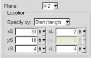 and the free area ratio is set to 0.5 as demanded in the given problem and put under the CEILING-RETURN Groups.
Created two rows of return grilles by copying the CEILING-RETURN Groups node and setting the Number of copies to 2, checking Translate, and setting the Z offset to 9 ft. Copied the CEILING-RETURN Groups node again Checked to Translate and set the X offset to -14 ft to create the second row of return grilles.
Created two more return grilles just above CRAC units by selecting the grille command and modifying the dimensions as given below:
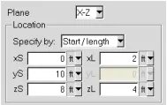
In the Info tab, it was named ceiling-return-crac1 under the Name section and put into CEILING-RETURN from
the Groups drop-down list, and the Properties tab, the Free area ratio is set to 0.5.
Ceiling-return-crac1 from the Model tree was copied and put into the CEILING-RETURN group created.
Checked to Translate and set the Z offset to 10 ft, and renamed it as ceiling-return-crac2.
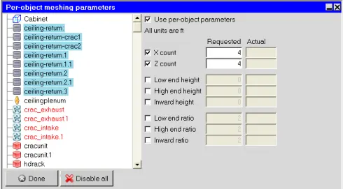
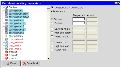
Per-object meshing parameters are set as shown below:
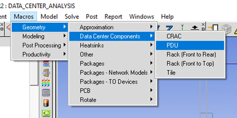
Creation of a PDU
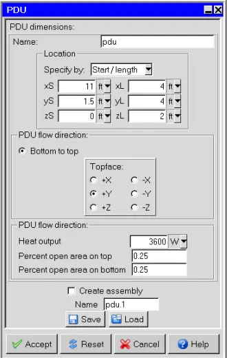
PDU is created as shown below:
The per-object meshing parameters for the grilles pdu_vent_in and pdu_vent_out are set by opening the Mesh control panel by clicking the Generate mesh button and by editing the local tab value, and the X count and Z count options are set to 4.
Created a new group for the PDU named as PDUs by selecting pdu_unit and then pdu_part4 in the Model Manager window.
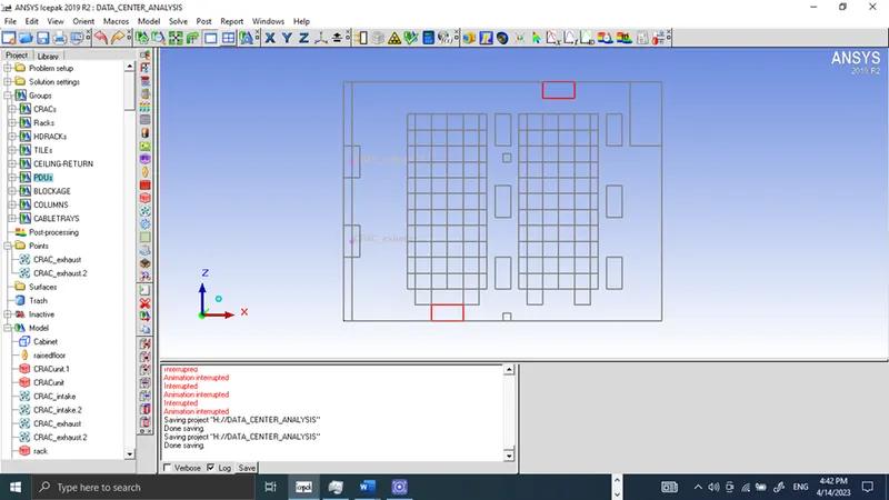
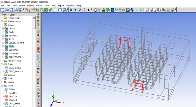
Created the second PDU by copying the PDUs in the Groups node and checked to Translate and set the X offset to 14 ft and the Z offset to 28 ft. PDUs are shown in red color in the image given below:
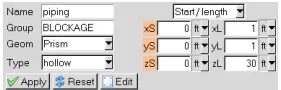
A blockage named piping is created by using a block object and put into the BLOCKAGE group as shown below:
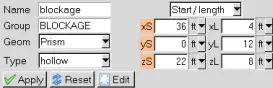
Another blockage is created by the method given above and shown in the image given below:
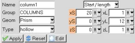
A column named column1 is created by using a block object and put into COLUMN as shown below:
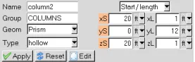
another column as column2 is created and put into the COLUMN group as shown below:
A cable tray named cabletray1 is created by using a block object and put into the group CABLETRAYS as shown below:
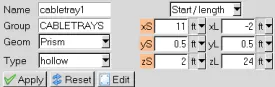
Created three more cabletrays by copying CABLETRAYS in the Groups node and checked to Translate and set to the X offset to 6 ft, and again copied CABLETRAYS in the Groups node and Checked to Translate and set to the X offset to 14 ft.
The completed data center model is shown below:
Mesh Generation
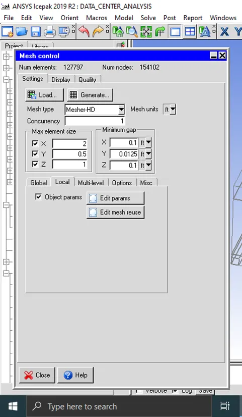
by Clicking on the Generate mesh button and putting element size and minimum gap dimensions as shown below, a good quality mesh is generated.
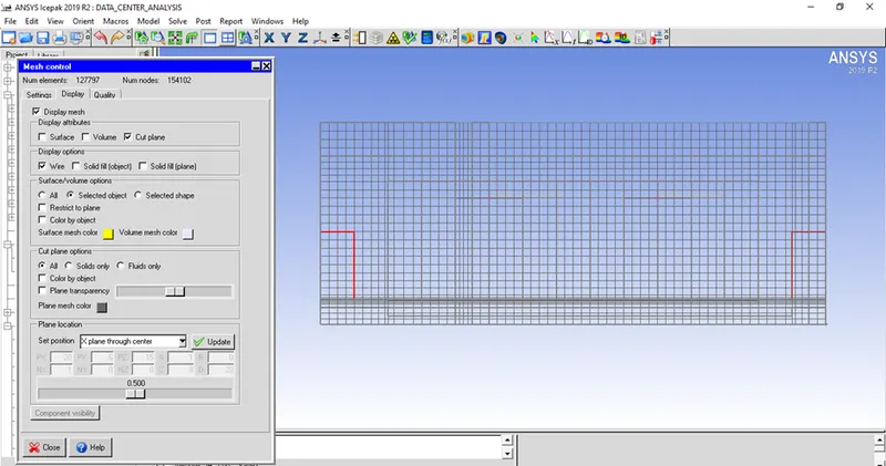
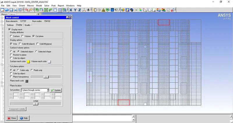
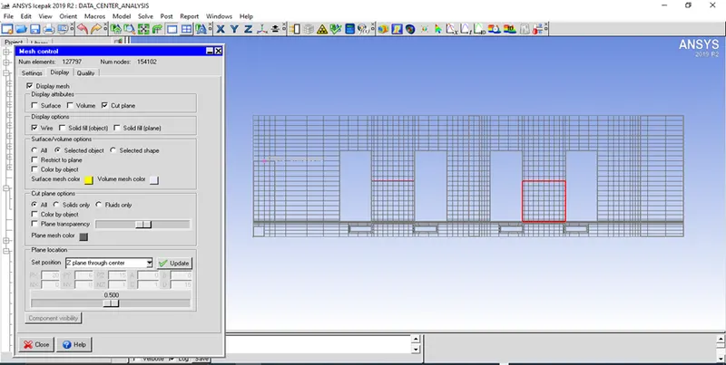
The quality of a generated mesh can be observed in the different cross-sectional planes as given below:
Mesh quality in the X plane through the center.
Mesh quality in the Y plane through the center.
Mesh quality in the Z plane through the center.
Mesh quality in terms of face alignment, volume, and skewness.
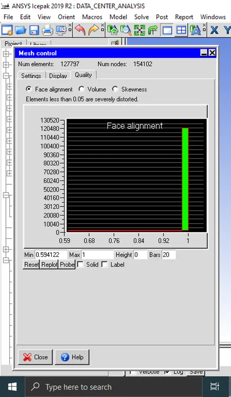
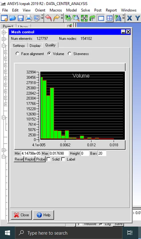
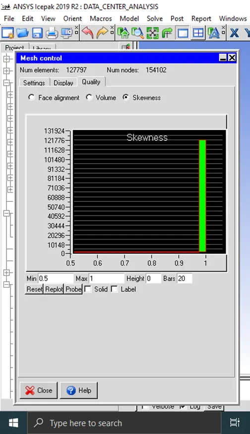
From the above mesh cut plane and mesh quality plots, it is clear that generated mesh is of good quality and now the model is ready for further processing.
Creating Monitor Points
Created two temperature monitor points for the CRAC fans exhaust fans named crac_exhaust
and crac_exhaust.2 from the Model node to the Points node. The default setting is to monitor Temperature, Pressure, and Velocity.
Physical and Numerical settings
In the problem setup, basic parameters are set to solve flow and temperature variables, radiation is kept off, the flow regime is selected as turbulent, and the zero equation is selected for turbulence modeling. Gravity is kept on. The general setup is shown below: 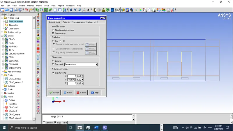
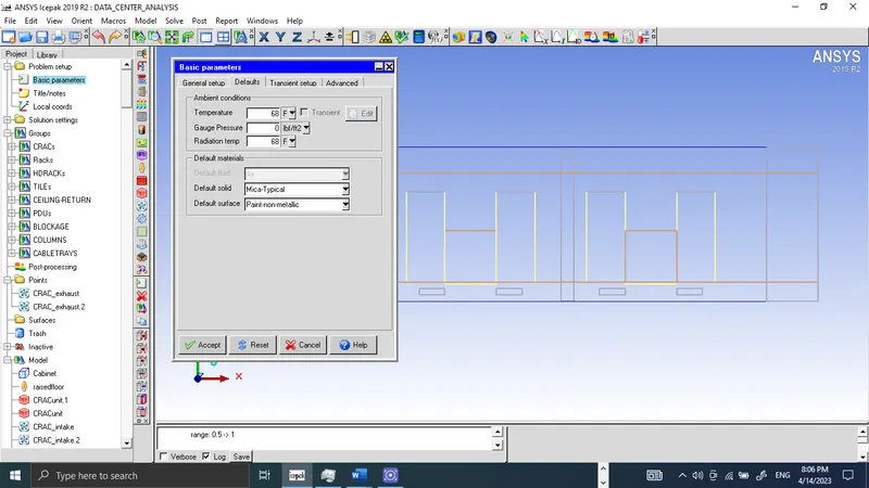
Parameters selected under the defaults tab are shown below:
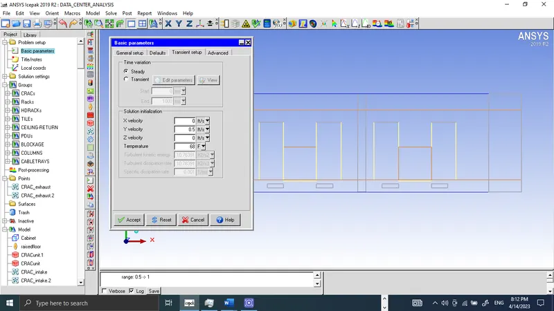
The initial Y velocity is to be 0.5 ft/s. It is recommended for problems
involving natural convection. The transient setup used is shown below:
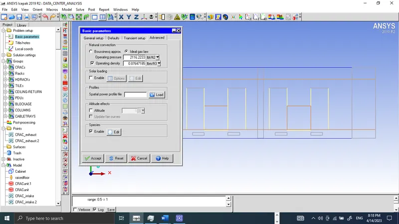
The Advanced tab is set for the Ideal gas law. It is recommended for problems involving significant temperature differences. The Operating density is kept as the default value. the Species is enabled and kept as default values in the Species Definitions panel.
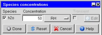
 The RH value for the crac-intake fans is set as given below:
by clicking crac_intake and then crac_intake.2 in the
Model manager window, and by selecting Edit from the context menu, under the Fan’s [*multiple*] Properties tab Edit is selected and under the Species concentrations panel, RH from the concentrations list is selected and the value entered is 50.
Under solution settings, the basic setting is selected and the number of iterations is set to 1000, and the convergence criteria for energy is set to 1e-6.
Under the Advanced settings, the Discretization scheme is set for Pressure as Body Force Weighted.
and the Under-relaxation to 0.2 for Momentum and 0.1 for Body forces.
Now after saving the model solution is run.
Results using different types of plots and animation.
Solution residuals and monitor plots are given below:
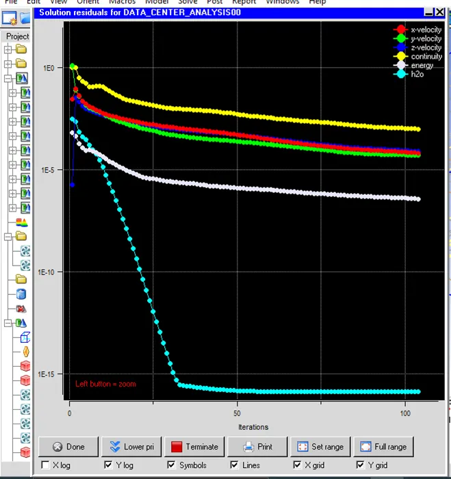
From solutions residual plots, we can verify that the solution is conversing after 100 iterations.
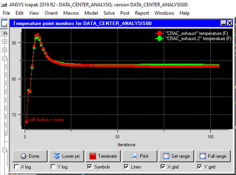
Temperature monitor points plot for CRAC_exhaust, and CRAC_exhaust.2 vs the number of iterations shows maximum temperature is reached above 90 degrees Fahrenheit. When the steady state is reached maximum temperature is around 84 degrees Fahrenheit.
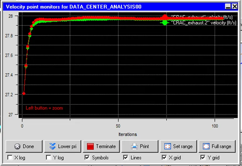
Velocity monitor points plot for CRAC_exhaust and CRAC_exhaust.2 vs the number of iterations shows maximum velocity is reached around 28 ft/s.
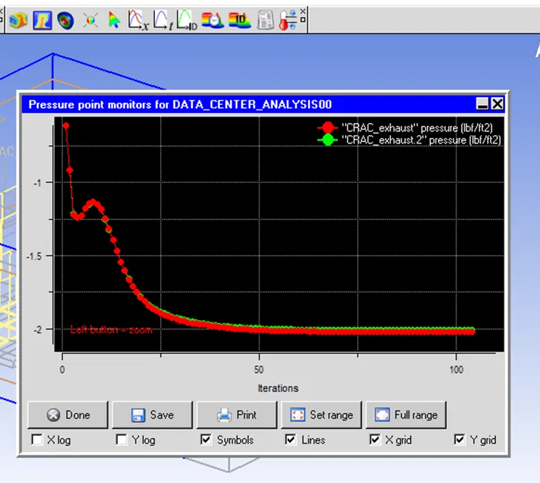
Pressure monitor points plot for CRAC_exhaust and CRAC_exhaust.2 vs the number of iterations.
Object Face Temperature Contours.
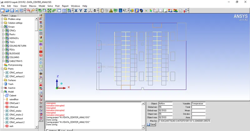
From the Object's Face Temperature Contours plot, it is clear that the temperature is lower on the side where cold fluid flows, and heat dissipates from the other side of the rack. The maximum temperature achieved is around 92.51 degrees Fahrenheit.
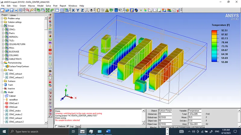
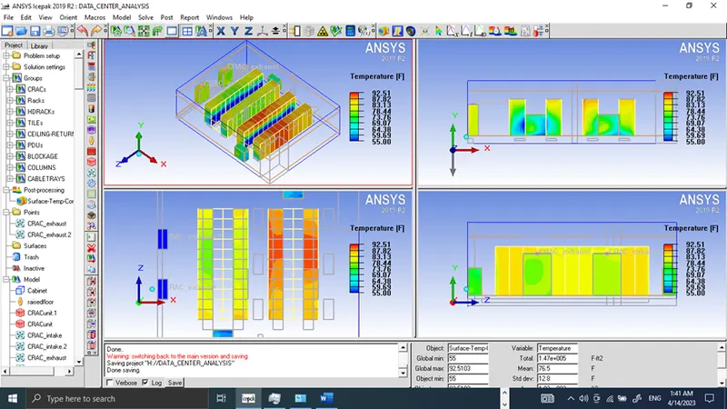
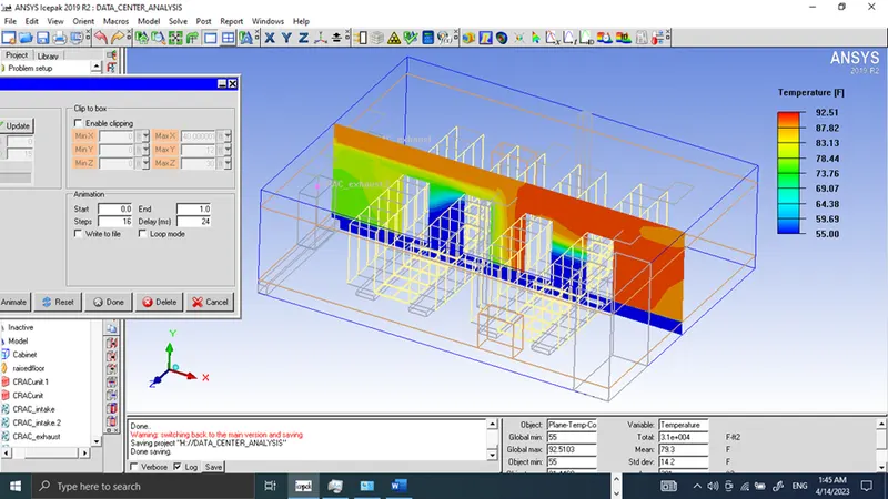
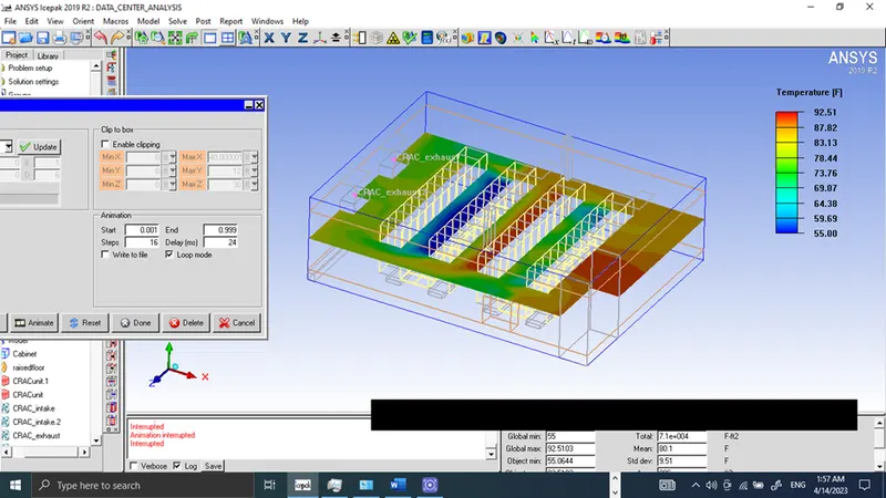
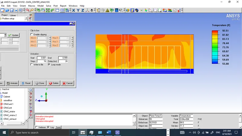
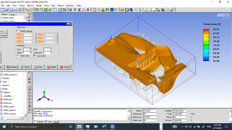
The above image of an Iso surface of temperature distribution shows how a particular temperature is distributed along the flow path.
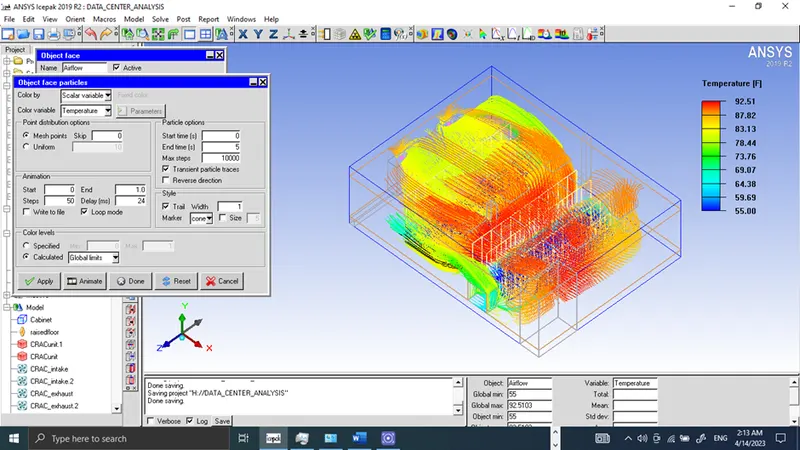
Particle trace plot shows where low-temperature streams are emerging from, how they are cooling the server racks, and what path they follow when getting hot.
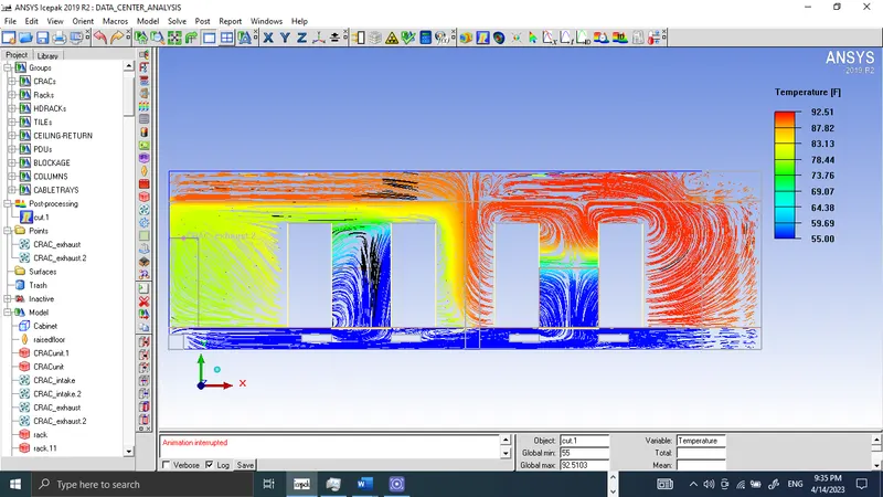
This plot shows how cold streams are emerging from tiles between the gaps of two server racks, cooling the servers, getting hot, and flowing towards CRACs.
Conclusions:
Datacenter modeling by using Macros is done as specified in the given problem.
The model is solved for flow, and temperature variables, and the flow regime is used as a turbulent flow (Zero equation model) while keeping the radiation effect off.
The face objects plots show how temperature is distributed, the maximum temperature reached is 92.51 degrees Fahrenheit, and the lowest temperature is on the side of tiles from where the cold stream is emerging.
YouTube links for the Animation plot are given below: