Week 5.1 - Non-Conformal Meshing and Solving a Cold plate model
Aim: To perform non-conformal meshing and do an analysis of two hot plates cooled by water circulating inside the cold plate cavity and also by air externally by natural convection.
Objectives:
- To create geometry
- To do non-conformal meshing
- To set up the physics model
- To examine and post-process the results
1. Geometry Creation
a. Cabinet of a given size is created by modifying the built cabinet geometry available with ICEPAK.
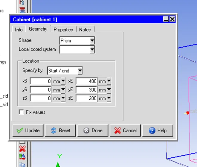
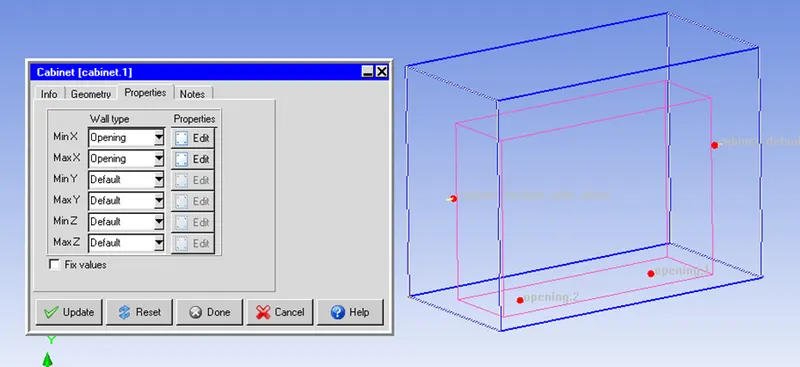
The minimum and Maximum X of the cabinet is kept open.
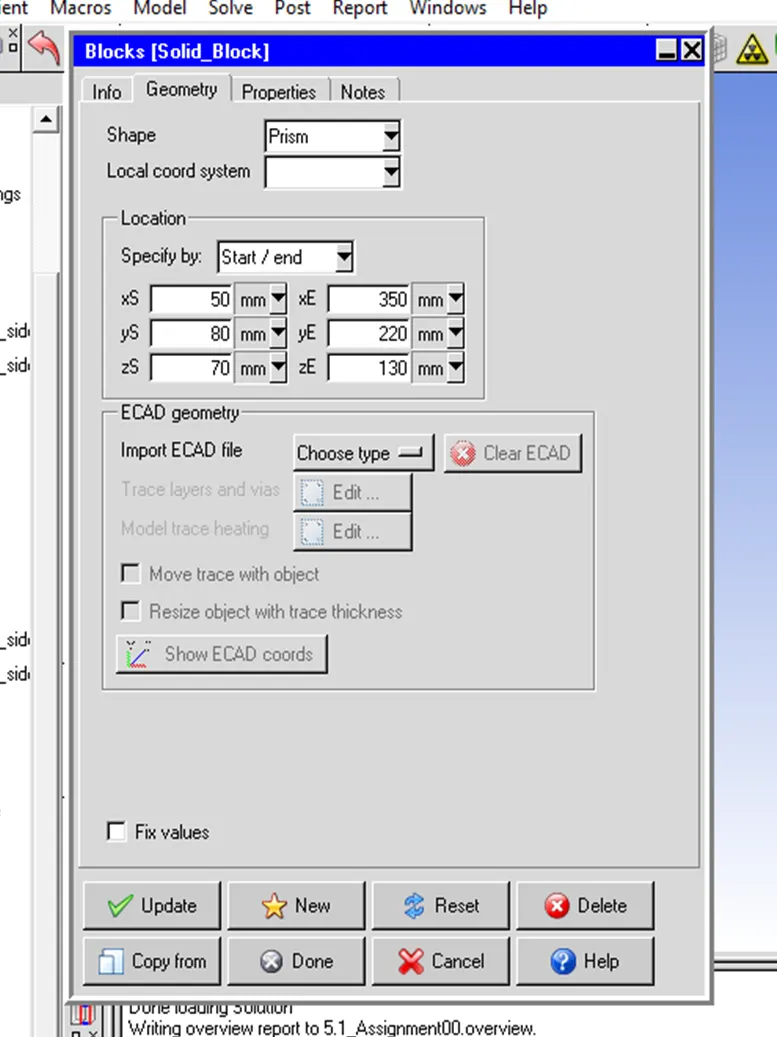
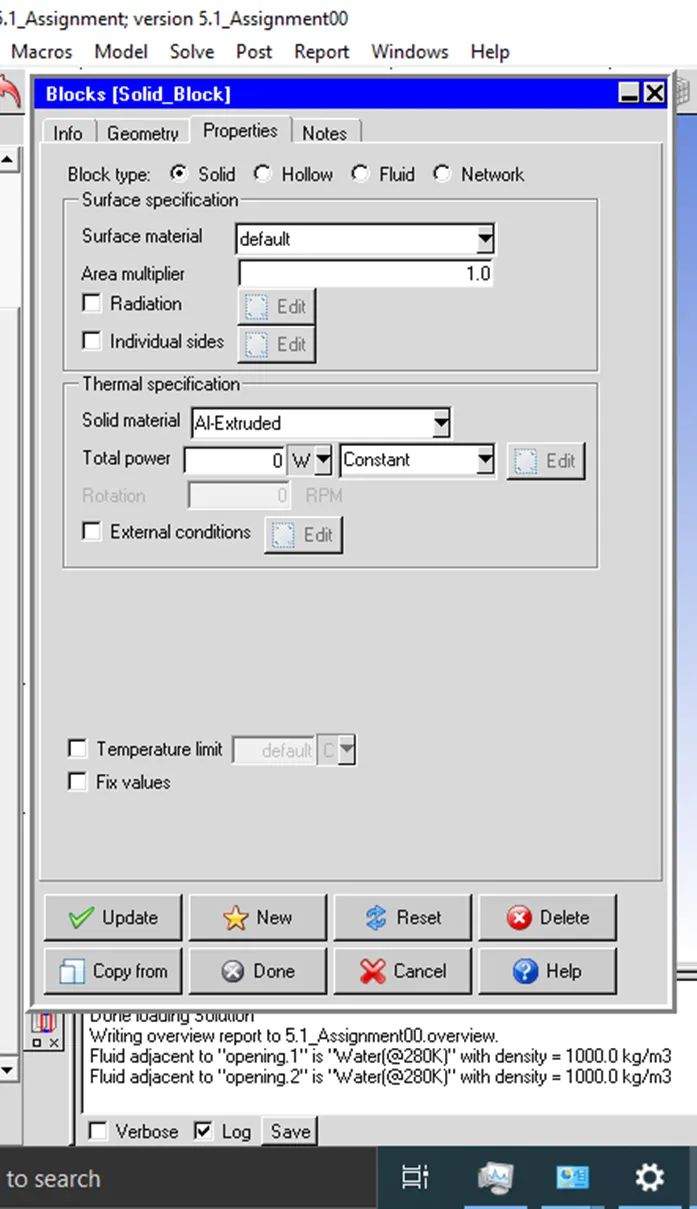
Solid block, solid inlet, and solid outlet pipe materials are Al-Extrude.
Solid Block geometry.
Solid Block Properties
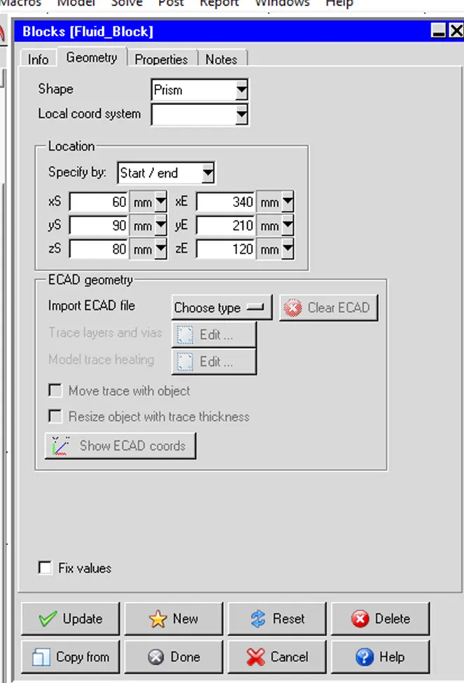
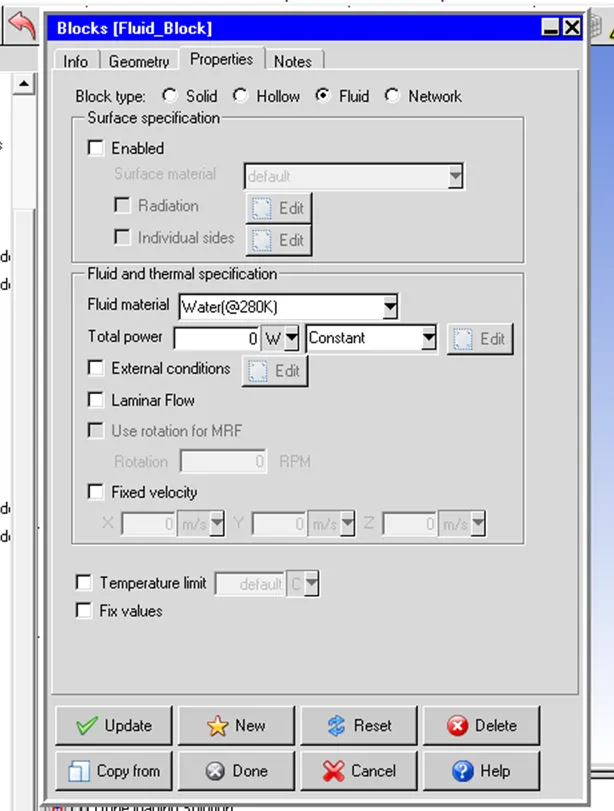
Fluid Block Geometry and its material is given below.
Properties of Fluid Block.
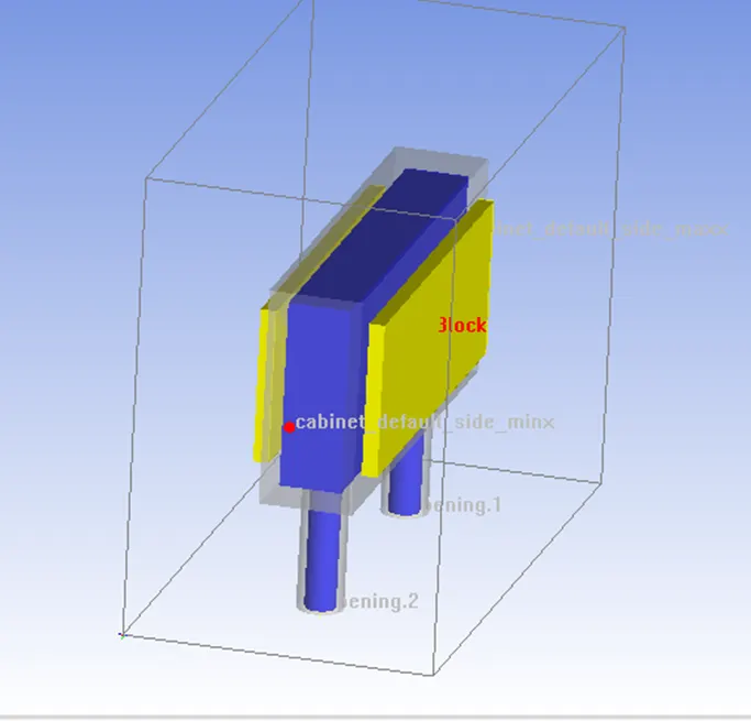
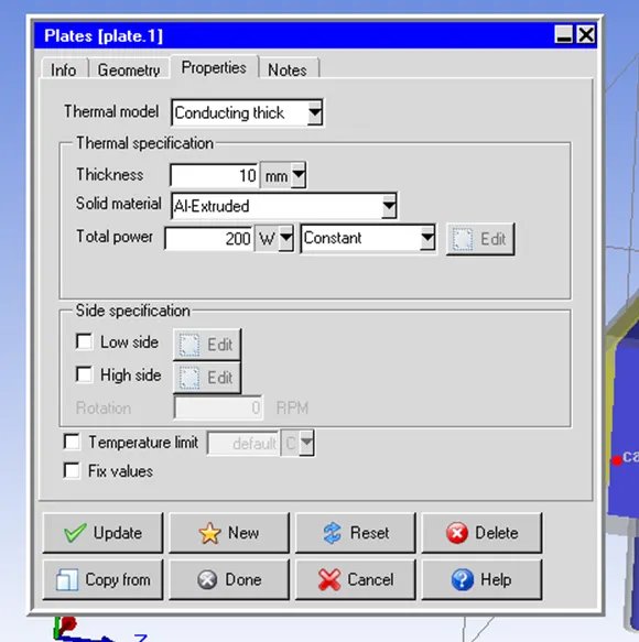
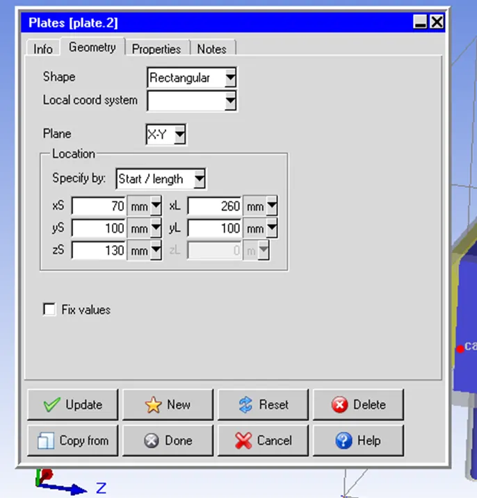
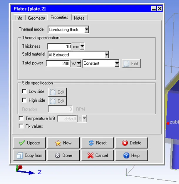
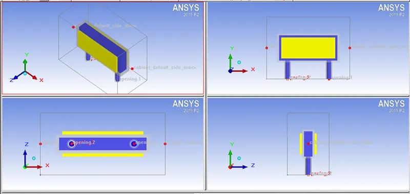
Hot Plates 1 and 2 are made of Al-Extrude of 200 W of each for heat generation. The type of Plates is Conducting Thick and each is made of Al-Extrude, and plates have been placed on both sides of a solid block as shown in the image below.
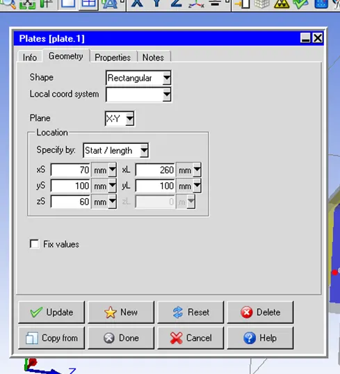
Dimension of Hot Plate 1.
Properties of Hot Plate 1.
Geometry and Properties of Plate 2.
The Geometry of Solid Inlet and Outlet Pipes are given below.
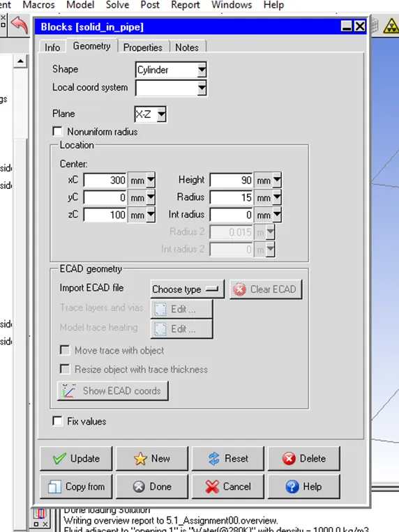
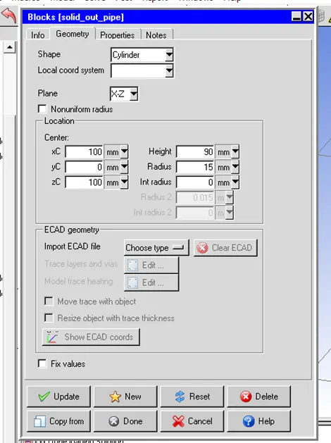
The geometry of Fluid Pipes.
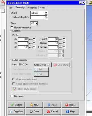
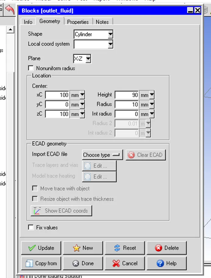
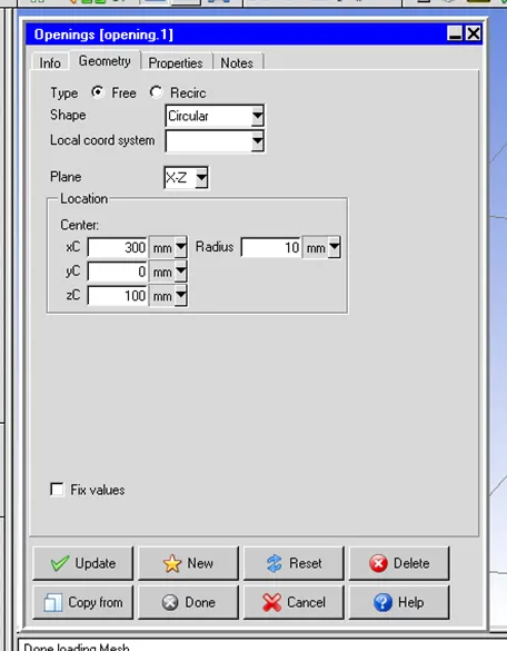
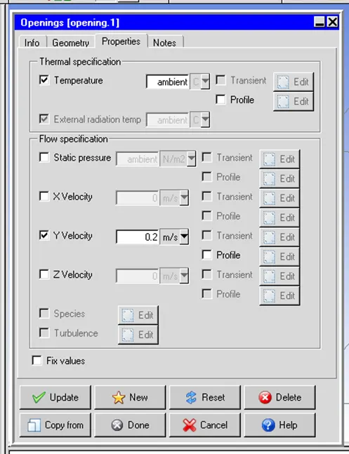
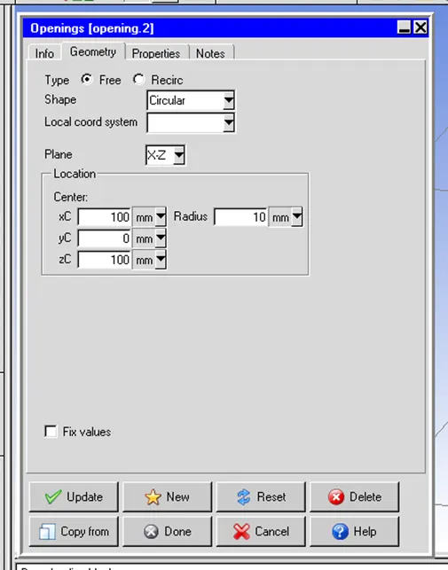
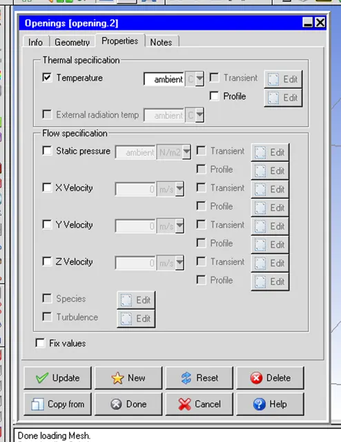
Pipes' Openings and Their geometries are given below. The Inlet Pipe opening is given a velocity of 0.2 m/s in the positive Y direction.
Inlet Opening Geometry.
Inlet Opening Properties.
Outlet Opening Geometry.
Outlet Opening Properties.
Completed geometry of the cold plate problem.
2. Non-Conformal Meshing
Non-Conformal meshing is performed to avoid mesh bleeding while maintaining the same level of accuracy and mesh resolution.
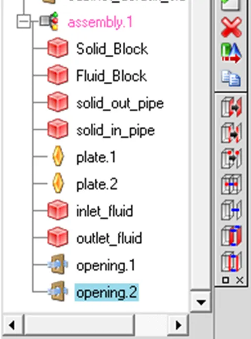
To perform non-conformal meshing, an assembly is created using the following objects given below:
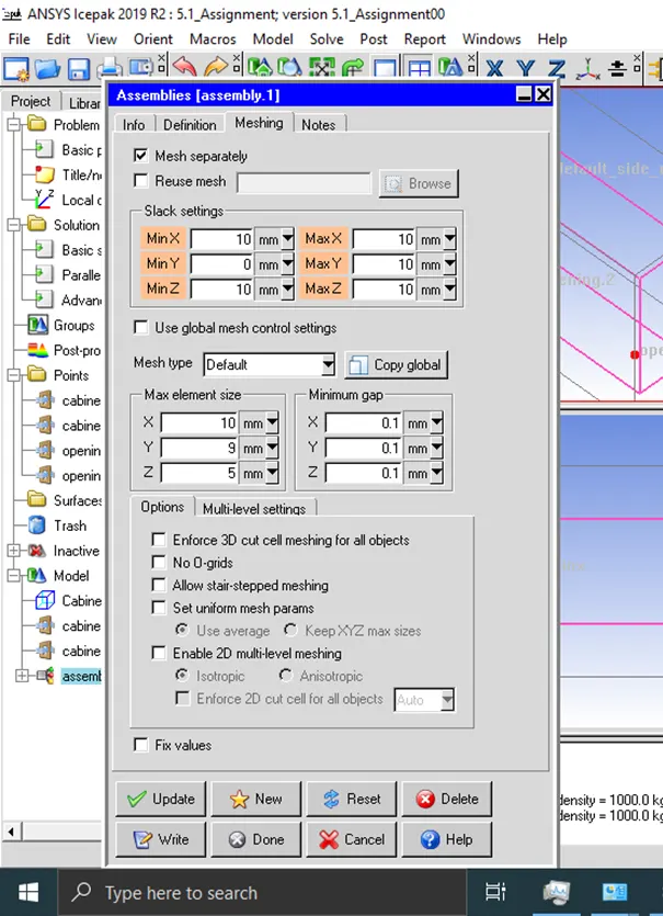
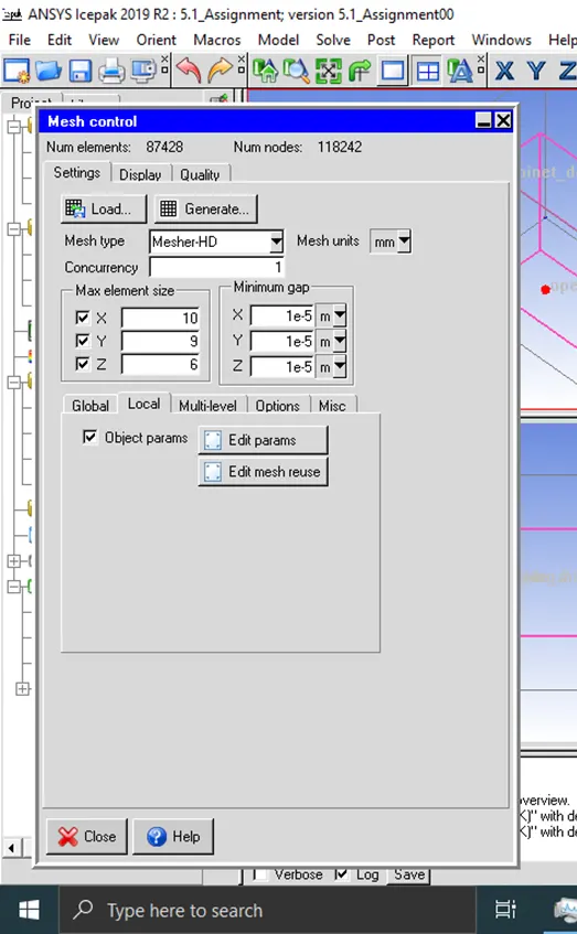
Mesh settings applied for Assembly meshing and mesh control are given below.
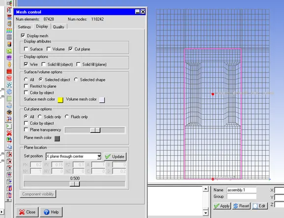
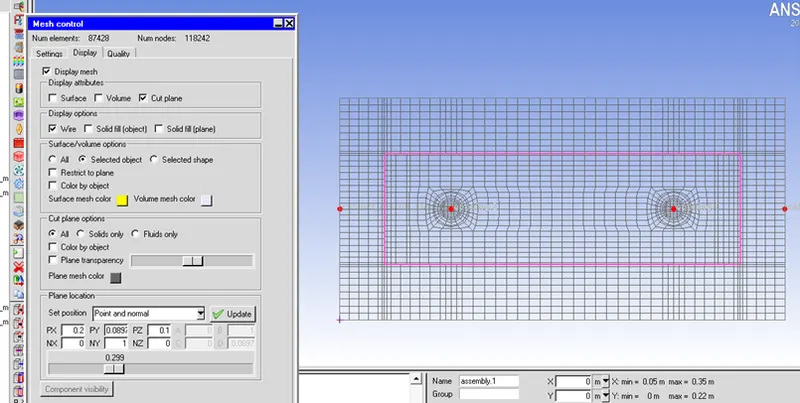
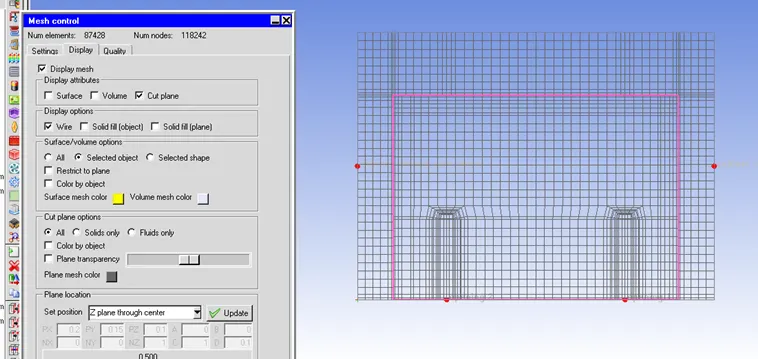
Quality of mesh along shown in different cut planes as given below.
Mesh along X Plane through the center.
Mesh along Y Plane through the center.
Mesh along Z Plane through the center.
Mesh Quality in terms of Face Alignment, Skewness, and Volume.
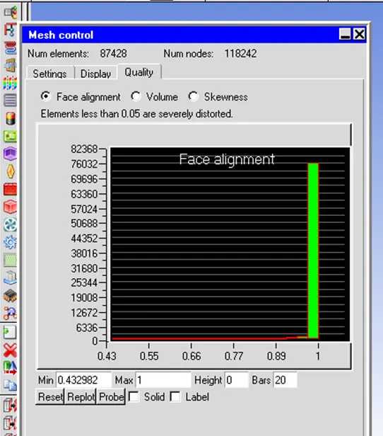
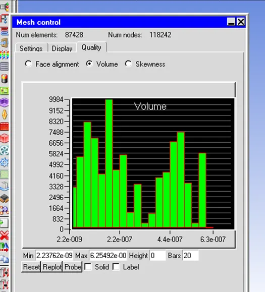
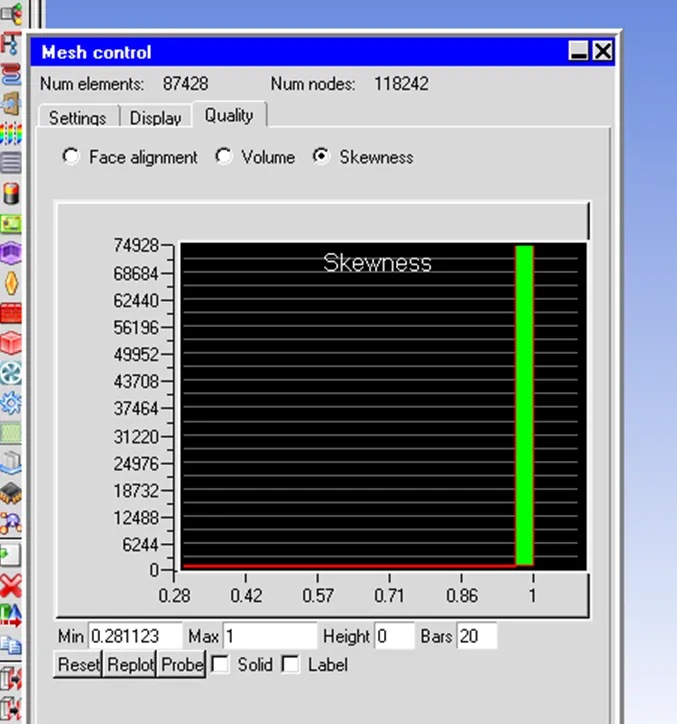
The above-given quality check shows that the mesh generated is of acceptable quality and can be used to perform the intended simulation.
3. Setting Up Physics Model
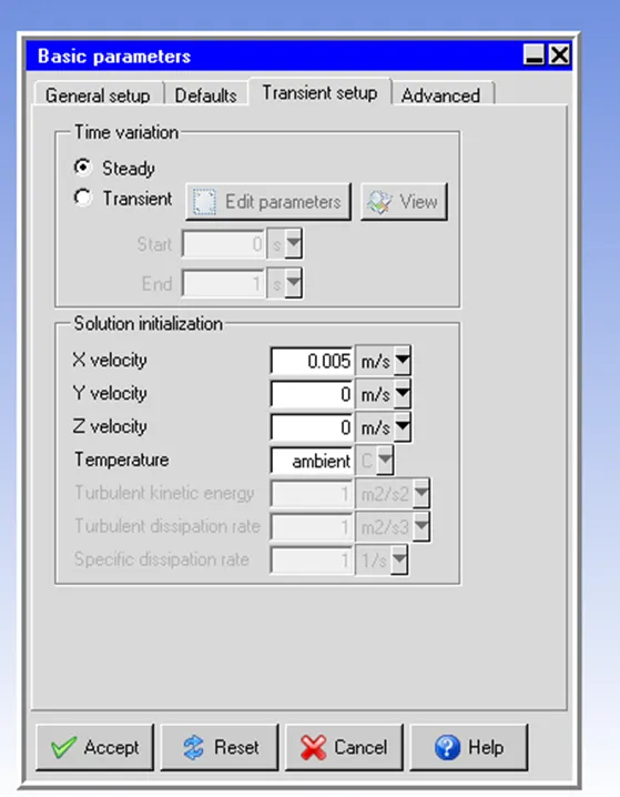
The model is to be solved for steady flow and temperature variables and the radiation effect is neglected. The zero equation of the turbulence model is to be solved for the flow regime. The gravity effect is taken in the x direction of the given domain as g = -9.81 m/s2. A small velocity of 0.005 m/s2 is given in the anti-gravity direction to initialize the solution process.
Ansys ICEPAK uses Ansys Fluent Solver to solve the Navier-Stokes equation in the given domain.
Model setup to solve the given model.
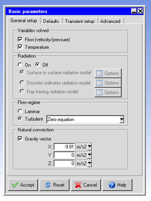
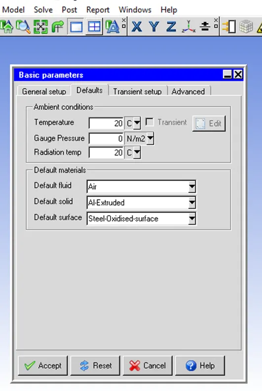
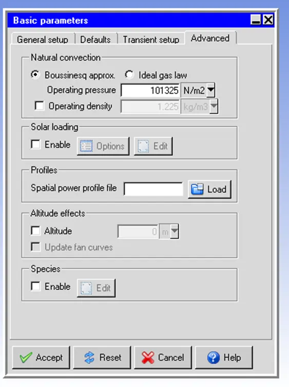
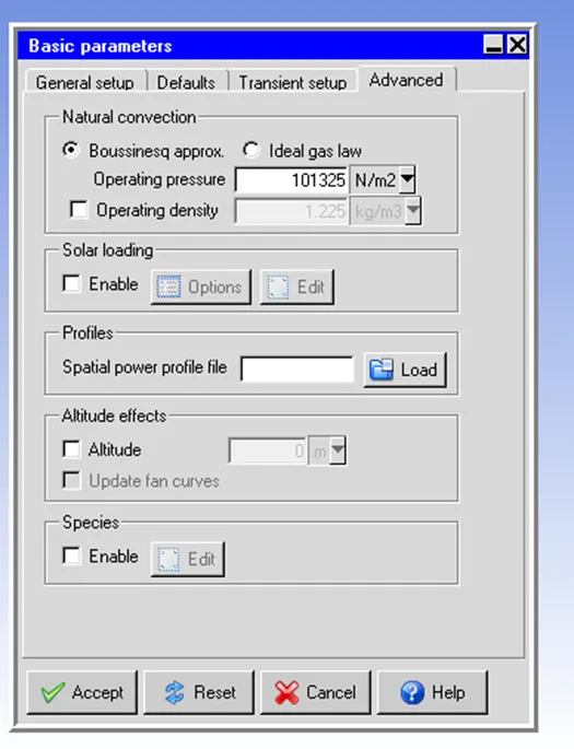
The Boussinesq approximation is applied to problems where the fluid varies in temperature from one place to another, driving a flow of fluid and heat transfer. The fluid satisfies the conservation of mass, conservation of momentum, and conservation of energy. In the Boussinesq approximation, variations in fluid properties other than density ρ are ignored, and density only appears when it is multiplied by g, the gravitational acceleration.
Solution Settings:
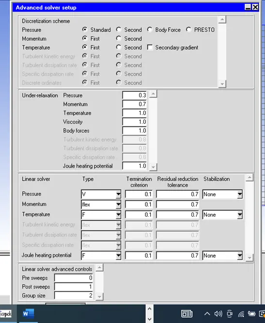
Settings used for solving the given problem are given below:

4. Examination and Post-processing of the results
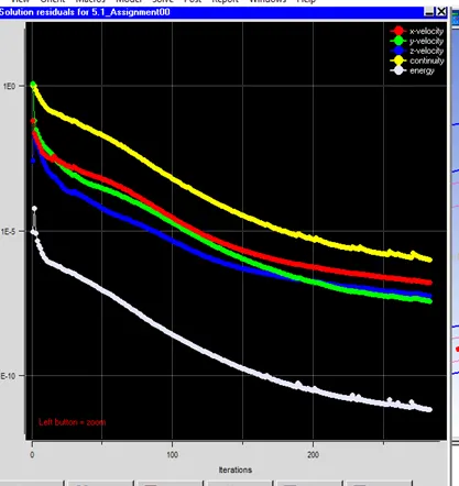
The residuals plot shows solution converses after 200 iterations, there is no change in the variables after 200 iterations.
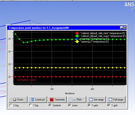
The monitor points plot shows the changes in the variables at particular locations with iterations. The monitor points work as probes that measure changes in variables.
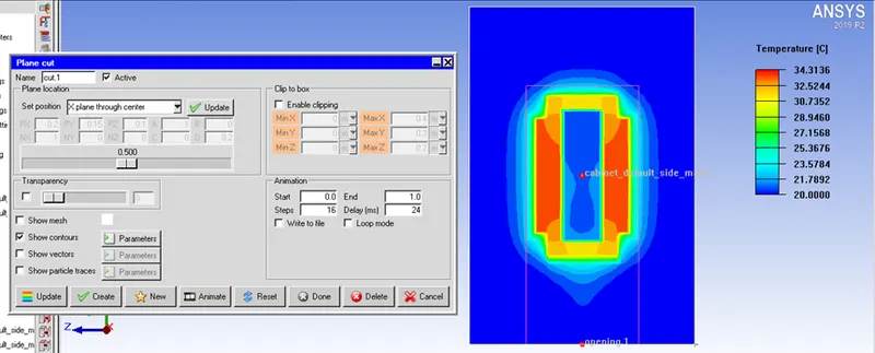
Temperature Contours in different planes
X-Plane through the center
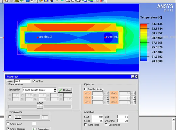
Y-Plane through the center
Z-Plane through the center
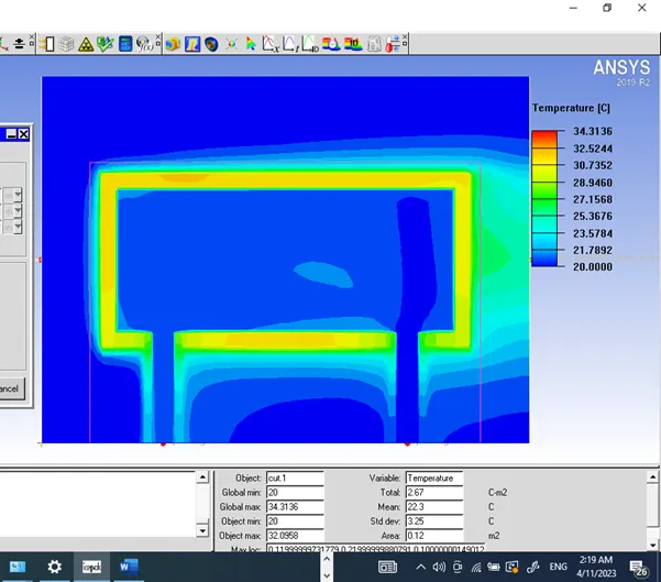
From the above plots, we can notice the air enters the cabinet at around 20 degrees Celsius, leaving out the cabinet at around 26 degrees Celsius, and water enters into the solid block at 20 degree Celsius. and leaves the outlet pipe at around 21 degree Celsius. A maximum of 34.31 degrees Celsius is attained inside the cabinet in the solid block and hot plates as shown on the contour plots.
Heat flows from higher temperature to lower temperature, which is evident from the contour plots. Hot plates are losing heat to the solid block and heat is dissipated to the water through natural convection. This is how hot plates are cooled. We can also notice the thermal boundary layer at the outer surface of the solid block.
Face temperature contours of solid and fluid blocks are given below to understand how heat is dissipated into different components of the model.
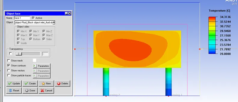
Temperature distribution inside the fluid blocks.
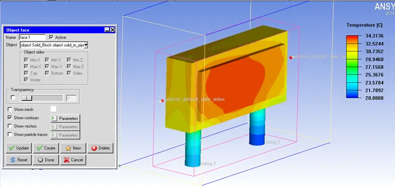
Temperature distribution inside solid blocks and hot plates.
Velocity contours are plotted to observe the distribution of velocity at a steady state in the model, which is given below.
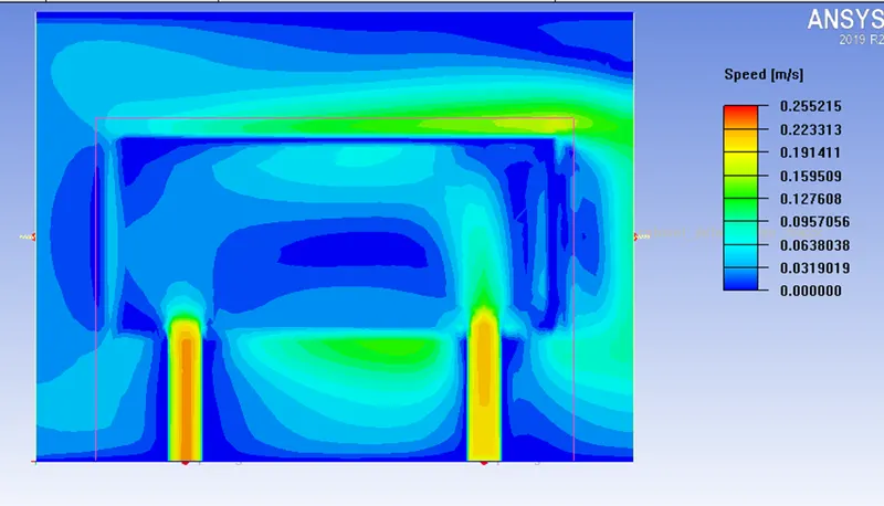
One can observe the convection cell around the solid block in a plane perpendicular to the XY plane. These convection cells are basically convection currents formed due to heat transfer between the solid block and ambient air inside the cabinet by the mode of Natural Convection.
Velocity Vectors in the different planes of the working domain are plotted to get further insights into the heat transfer mechanism of the cold plate model.
Z-Plane Velocity Vectors:
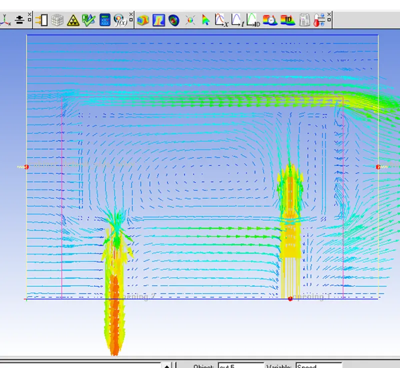
The above plot shows how fluid velocity is distributed inside the fluid block, inlet & outlet pipes, and outside the solid block, but it could not reveal convection currents formed which help in heat dissipation and maintain the temperature of the hot plates.
Animation of the same is given below:
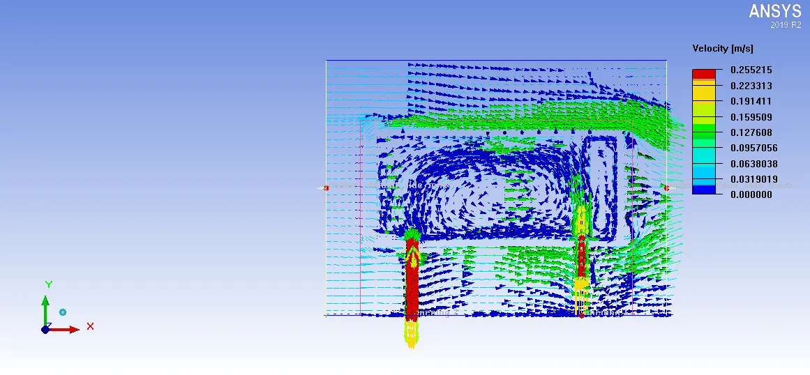
Animation of temperature Variation is given below.
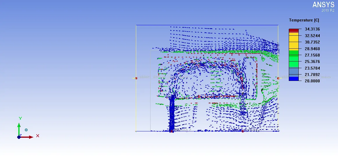
The Youtube link for the above animation is given below:
(Particle Tracing)
(Animation of temperature distribution)
Conclusions:
Simulation of cooling of hot plates by natural convection is done successfully.
Good quality of the non-conformal mesh is created for the analysis.
The following observations are made and given below:
Air leaves the cabinet at around 26 degree Celsius, and water leaves the solid block at around 21 degrees Celsius.
Convection currents are observed which show the cooling of hot bodies by natural convection.
The maximum temperature of the hot plates reached around 34.31 degrees Celsius, and the maximum temperature reached in the fluid block is around 33 degrees Celsius during steady-state conditions.