Week 10 - MRF project

Aim: To provide guidelines and recommendations for the Moving Reference Frame (MRF) fan modeling technique in ANSYS Icepak, and run a simulation for the same.

Objectives:

1. Modeling of the actual fan inside the cabinet.
2. Provide guidelines and recommendations for the Moving Reference Frame (MRF) fan modeling technique in ANSYS Icepak.
3. Meshing.
4. Problem Setup.
5. Postprocessing.

Answers:

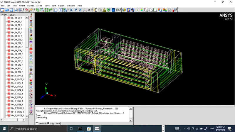
1st step is to open the given model in Ansys ICEPAK.

The model is open as shown in the image given below:

1. Modeling of the actual fan inside the cabinet.

Fluid Block Settings for MRF Setup

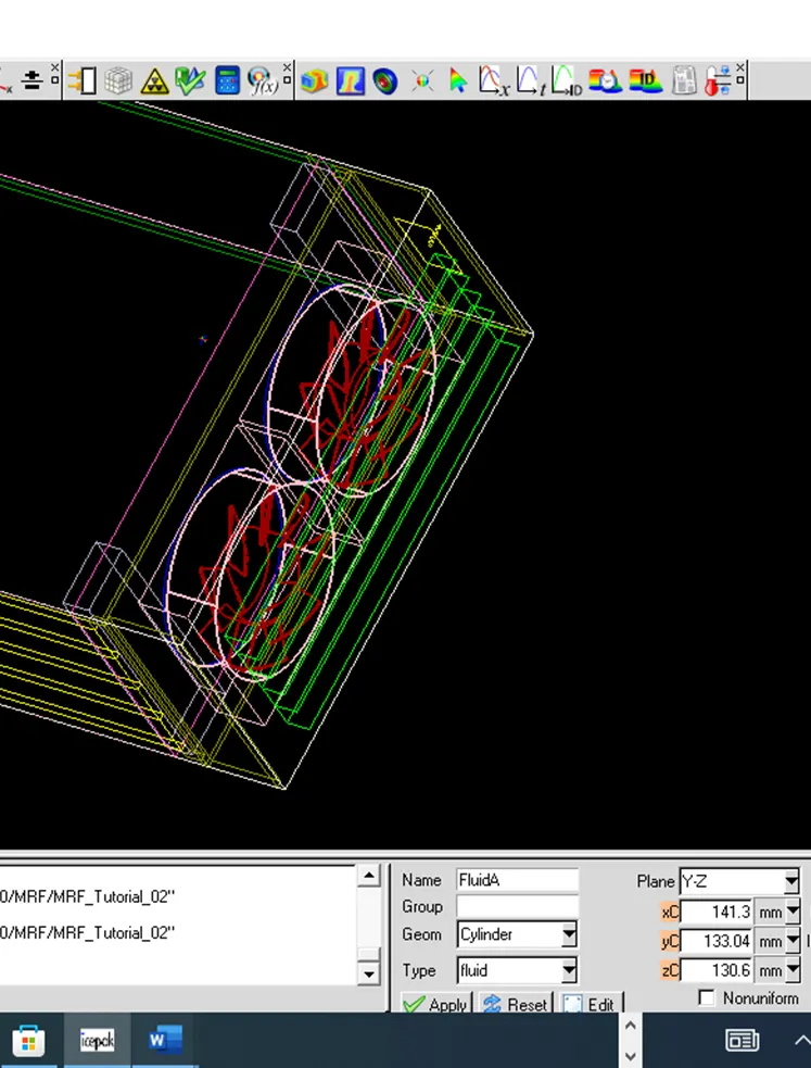
Two fluid blocks are to be created surrounding the fan blades and cutting through the casing blocks using the information given below:

Name	Shape	Plane	Center	Height	Radius	Type
FluidA	Cylinder	Y-Z	xc:141.3 mm yc:133.04 mm zc:130.6 mm	20	34	Fluid
FluidB	Cylinder	Y-Z	xc:141.3 mm yc:133.04 mm zc:56.6 mm	20	34	Fluid

Guidelines and recommendations for the Moving Reference Frame (MRF) fan modeling:

1. If the current object selection is not inside the assembly, the new fluid cylinders would
   appear outside and have to be dragged into the assembly.
2. The fluid cylinder blocks will be created at the bottom of the assembly list. This is because Icepak will, by default, give the newest objects the highest meshing priority. The fluid blocks need to have a higher priority than the case blocks but a lower priority than the fan rotor so that the rotor will have fully meshed. To automatically change the meshing priority, highlight these fluid cylinders in the Model tree, and drag them above the fan blades.
3. MRF is a technique used to model rotating equipment, such as fans, in CFD simulations. It involves rotating the fluid domain around the rotating equipment while keeping the equipment stationary.
4. Define the geometry of the rotating equipment accurately, including the fan blades, hub, and shroud. Create a solid body or an assembly of solids.
5. In Ansys ICEPAK, define a rotating region around the rotating equipment using the "Rotating Region" tool. Specify the fan's rotation axis, rotation speed, and rotation direction. This defines the MRF zone where the fluid will rotate along with the equipment.
6. Define the MRF properties, such as the density, viscosity, and specific heat of the fluid in the MRF zone. These properties should be representative of the fluid properties at the operating conditions of the fan.
7. Generate a high-quality mesh for the entire domain, including the MRF zone, using appropriate meshing techniques, such as structured or unstructured meshing, depending on the geometry and requirements of the simulation.
8. Using the exact fan blade geometry is critical for the accuracy of the MRF fan modeling technique. If the fan housing contains straightening vanes, these must also be modeled with their exact geometries.
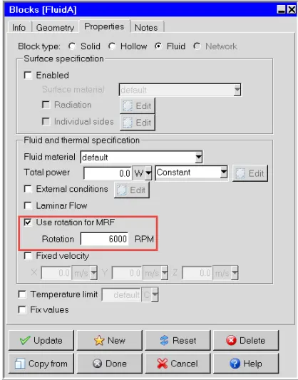
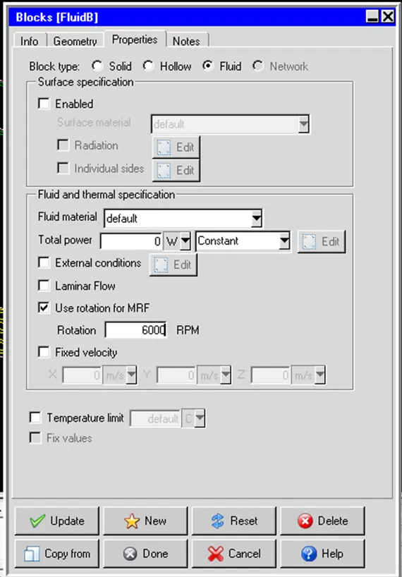
9. The rotation rpm here refers to the rotation of the fan rotor and blades. The direction follows the right-hand thumb rule.

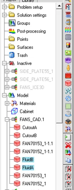
The created fluid block model is shown below:

MRF Settings:

Mrf settings for both fans are given below:

Mesh Generation:

HD meshing starts with a default hexa-unstructured mesh and progressively uses other element types in areas where geometric complexity does not allow for a good mesh with hexa elements. This “mesh mixing” occurs automatically in the meshing algorithm.

Proper resolution of CAD objects requires more mesh. Resolving surfaces with curvatures
typically requires more mesh than planar faces.

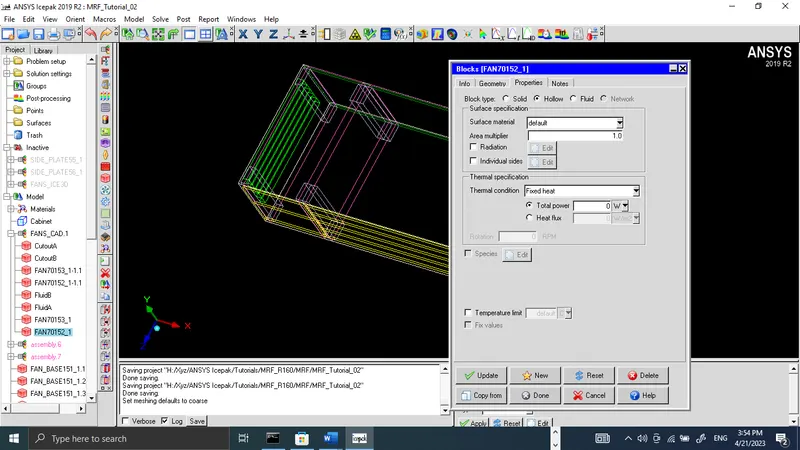
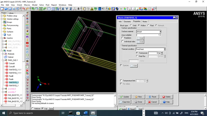
To keep the mesh count as low as possible, the Block type of the two rotor blocks (FAN70153_1–1.1
and FAN70152_1–1.1) are changed to Hollow.

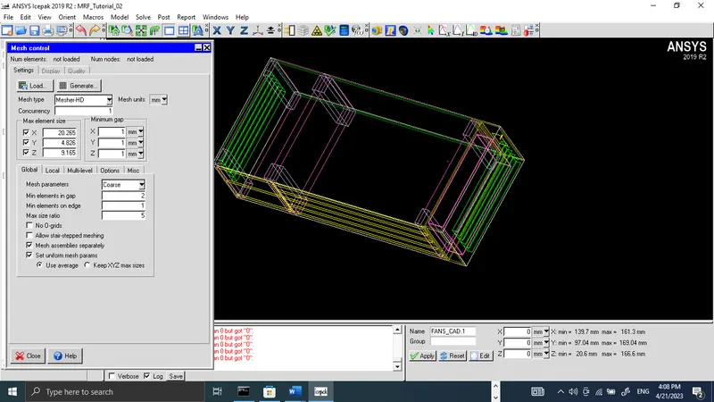
The global mesh setting is given below, the minimum gap in all directions is kept to 1 mm, and multilevel meshing is chosen up to level 2 only.

To restrict the finer mesh to the region immediately surrounding the fans, a non-conformal mesh should
be used.

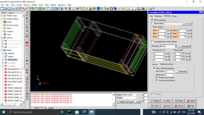
Settings for FANS_CAD.1 Assembly is given below:

Mesh Display and Mesh Quality:

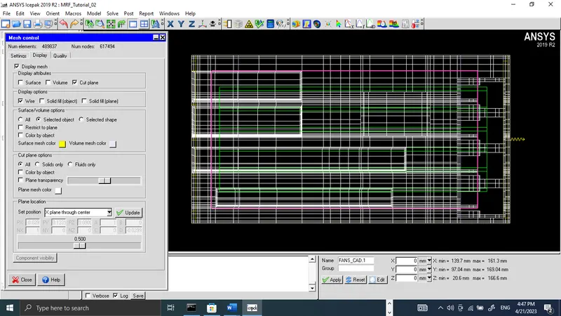
X Plane through the center of the cabinet

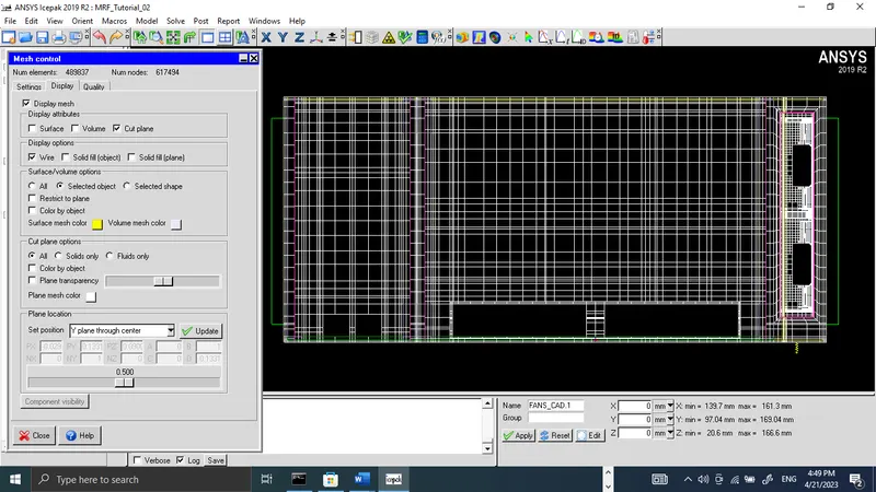
Y Plane through the center of the cabinet

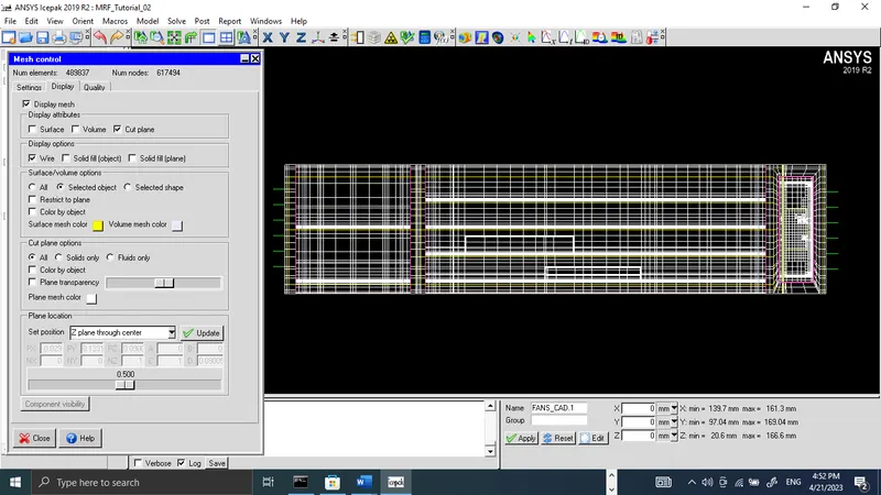
Z Plane through the center of the cabinet

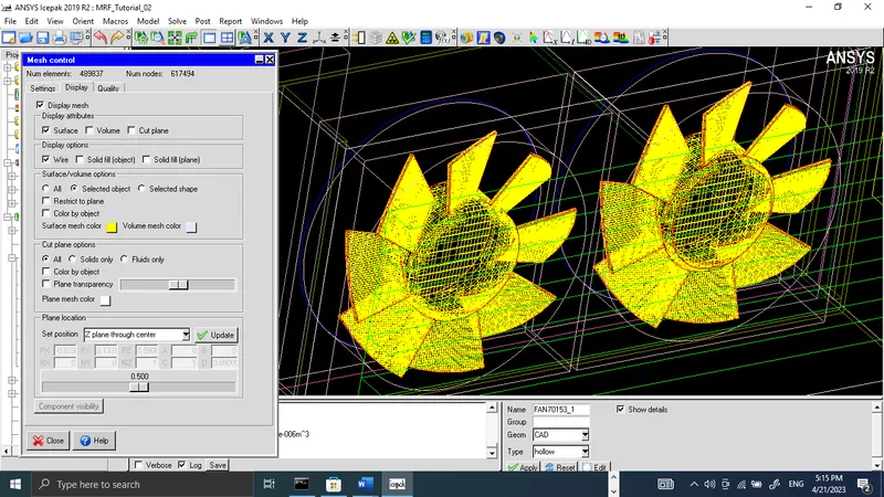
Surface mesh of Fans:

Mesh quality in terms of Face alignment, Volume, and Skewness is given below:

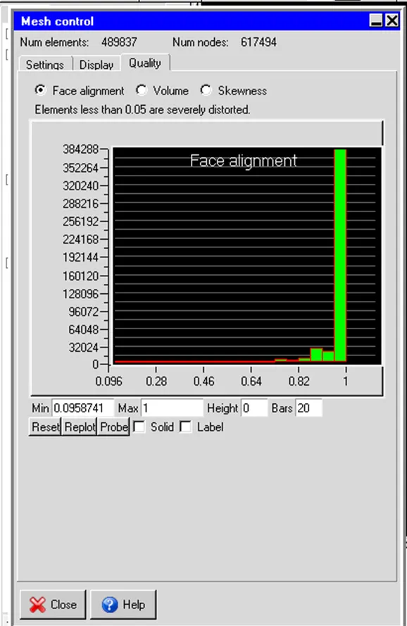
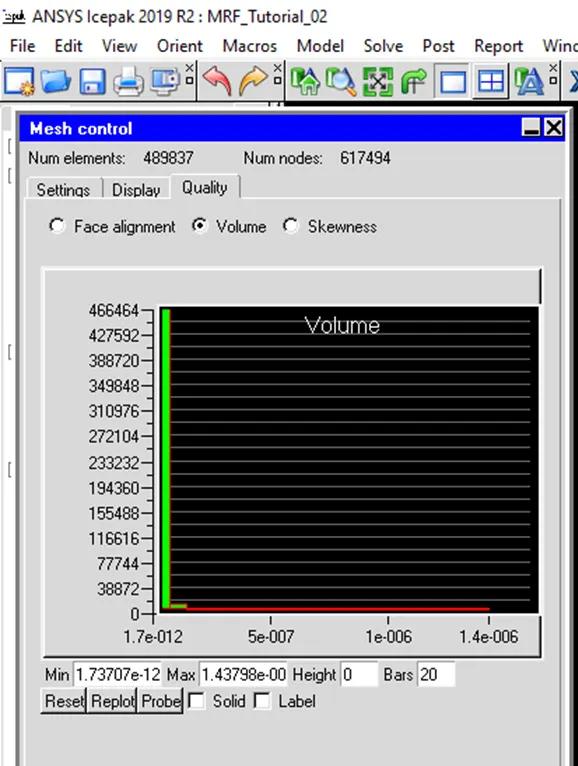
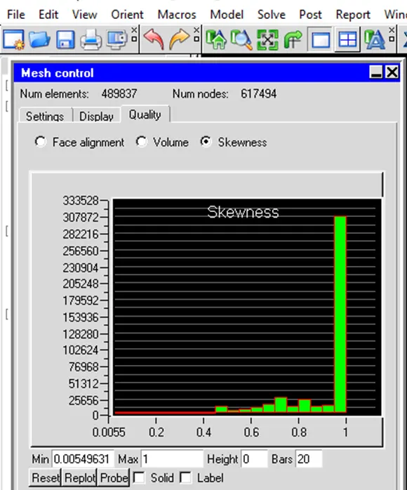
From the above plots, mesh quality is acceptable to get the first cut solution.

Physical and Numerical settings to run the simulation:

When running an MRF model, the zero equation turbulence model will not suffice as it does not properly
capture the swirl effects of the rotor blades. This is why the Realizable two-equation turbulence
model is used. The model is to be solved for flow and temperature variables. Radiation is kept off.

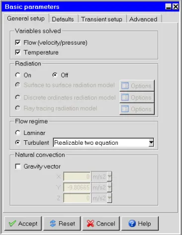
The Basic settings for convergence criteria and the number of iterations are given below:

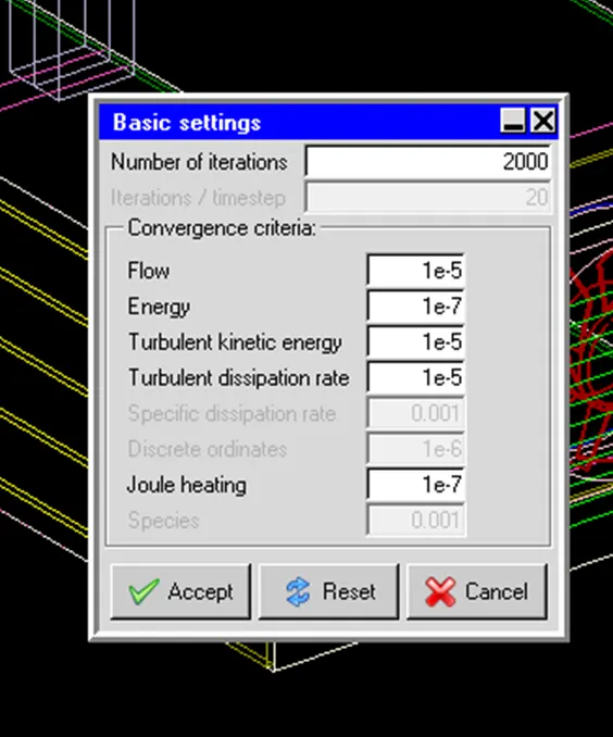
When using MRF, the solver typically needs a larger number of iterations to completely
converge. When running the initial solution it is recommended that you set the number
of iterations to something on the order of 2000 or more to see where the convergence
finally occurs.

Point Monitors:

The following monitor points are set as given below:

Point Monitor Location (X, Y, Z) mm Monitor
a. 163.3, 159.0, 62.41 Velocity
c. 172.7, 133.04, 93.6 Velocity
d. 163.3, 133.04, 110 Velocity
mon_pt_1. 172.7, 137.9, 135.3 Velocity
mon_pt_2. -232.6, 105.1, 98.5 Temperature
mon_pt_3. -232.6, 139.9, 79.99 Temperature
mon_pt_4. -219.5, 148.4, 26.85 Temperature

Results:

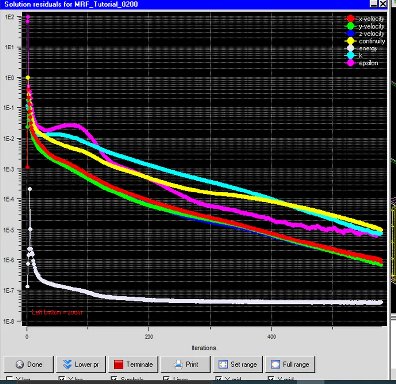
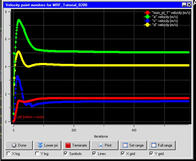
Solution residuals plot shows energy equation converges the first, steady state recahed after 200 iterations.

Monitor points for temperature shows after 200 iterations.

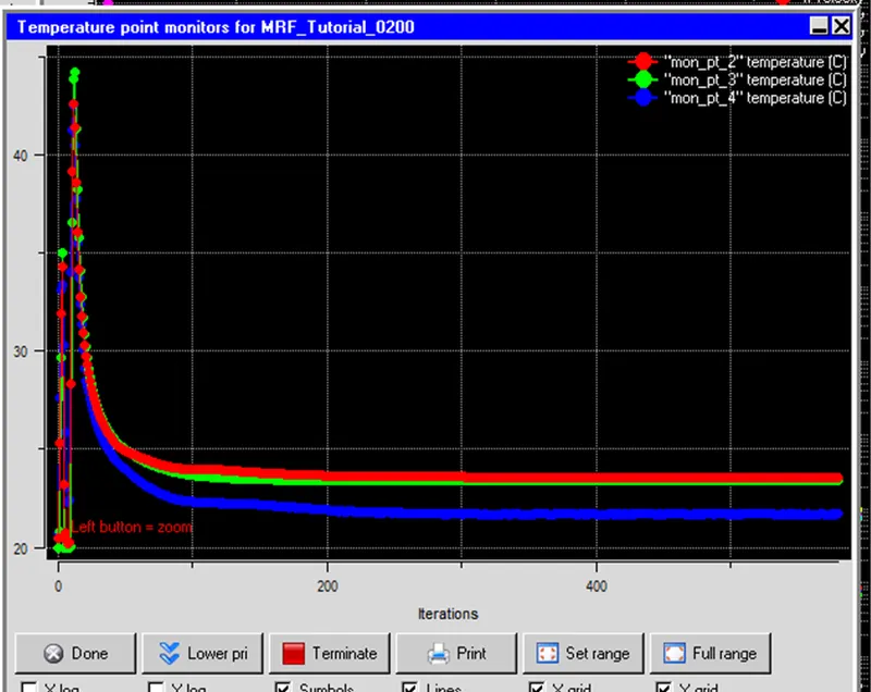
Monitors plot for velocity is given below:

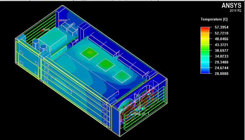
Object face temperature shows maximum temperature reached is 57.3954 degrees Celsius. Heat generating Bodies reached to the maximum temperature.

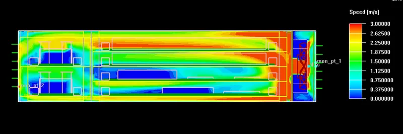
Velocity cut plot for the z plane passing through the center of the cabinet is shown below, velocities above 3 m/s are shown in red bands.

Conclusion:

Modeling of moving reference frame is done successfully while following proper guidelines and recommendations.

MRF modeling reduces errors in the calculation, and it is very useful in the analysis of turbulence flow, and system noise levels. This model is widely used in high density electronics models.