Week 6.2 - Setting up a model (Hanging Node)
Aim: To set up Hanging Node Model to study its thermal behavior.
Objectives:
- To load the already meshed model into Ansys Icepak
- To setup Physics and Numerical settings
- To analyze the results
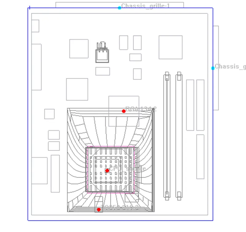
The loaded Model in Ansys ICEPAK is shown below:
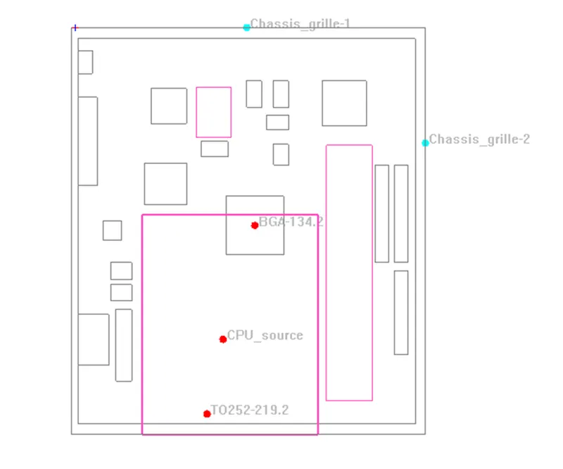
The model is ready with mesh assembly separately to perform non-conformal mapping to avoid mesh bleeding:
Generated Mesh cut plane is shown below, it shows a good-quality mesh that is ready for further analysis.
Z Plane Through Center
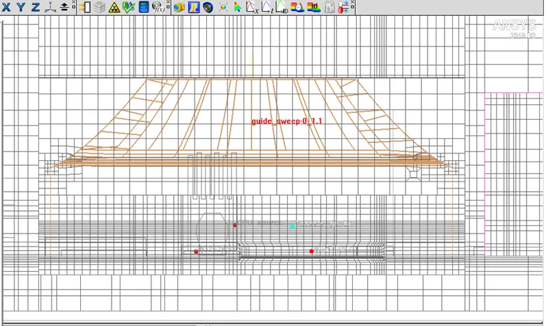
Y Plane Through Center
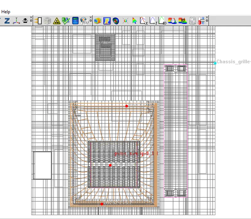
X Plane Through Center
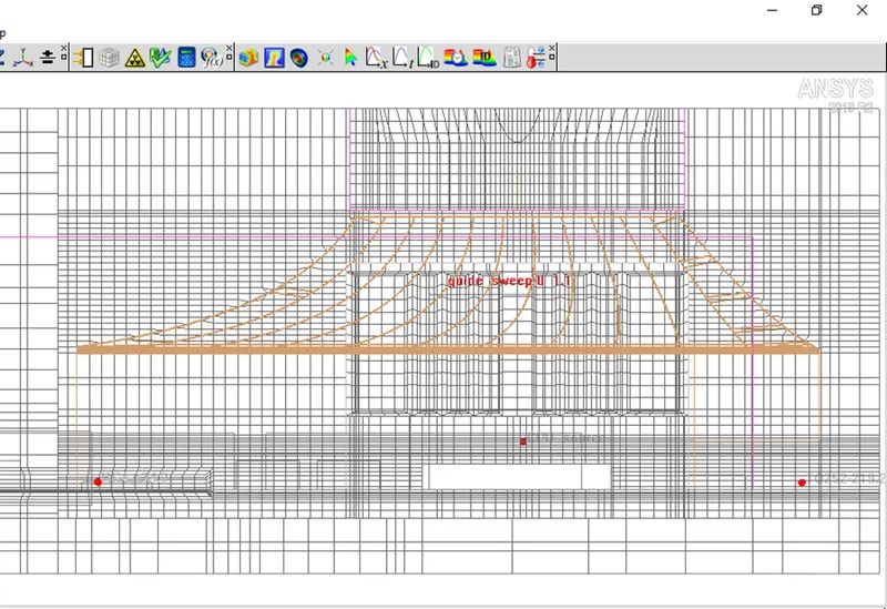
Multilevel Meshing:
Multilevel meshing is a technique used in computer-aided engineering (CAE) simulations to divide a complex geometry into multiple levels of smaller and simpler meshed regions. The idea behind multilevel meshing is to reduce the overall computational cost and improve the accuracy of the simulation results by using different mesh sizes in different regions of the geometry.
In multilevel meshing, the geometry is first divided into large regions, and a coarse mesh is generated for each of these regions. Then, each large region is subdivided into smaller subregions, and a finer mesh is generated for each of these subregions. This process can be repeated several times, with each level of mesh refinement creating a more detailed mesh of the geometry.
The advantage of multilevel meshing is that it allows the use of finer mesh resolution in areas where the simulation is most critical, such as near boundary layers or regions of high stress or strain. At the same time, it reduces the computational cost of the simulation by using a coarser mesh in areas where the simulation is less critical.
Multilevel meshing helps to improve the accuracy and efficiency of CAE simulations, particularly for complex geometries where a uniform mesh size may not be appropriate. In the current problem up, 2 levels of meshing are performed, and quality can be further improved but for the first cut problem, it is sufficient for now.
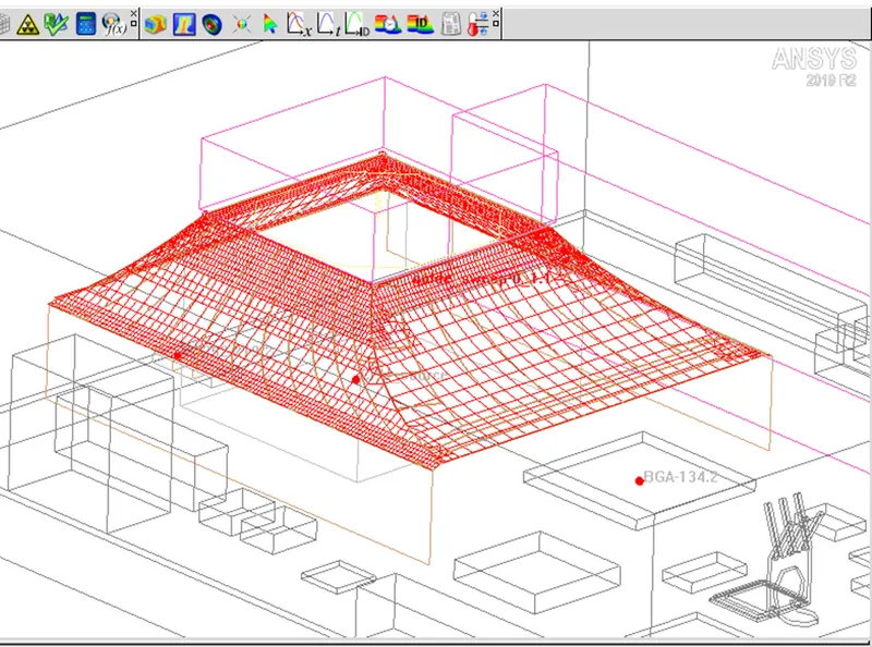
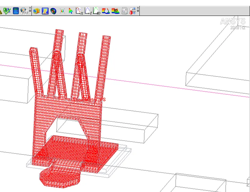
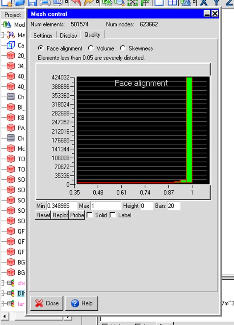
Quality of Mesh Plot
Face Alignment:
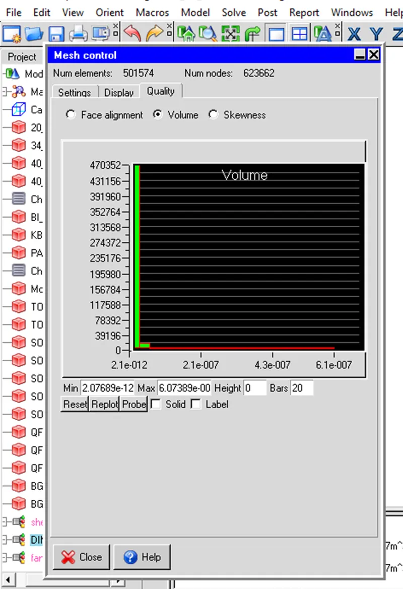
Volume:
Skewness:
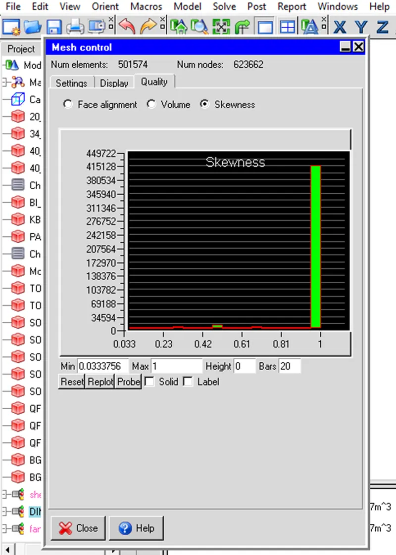
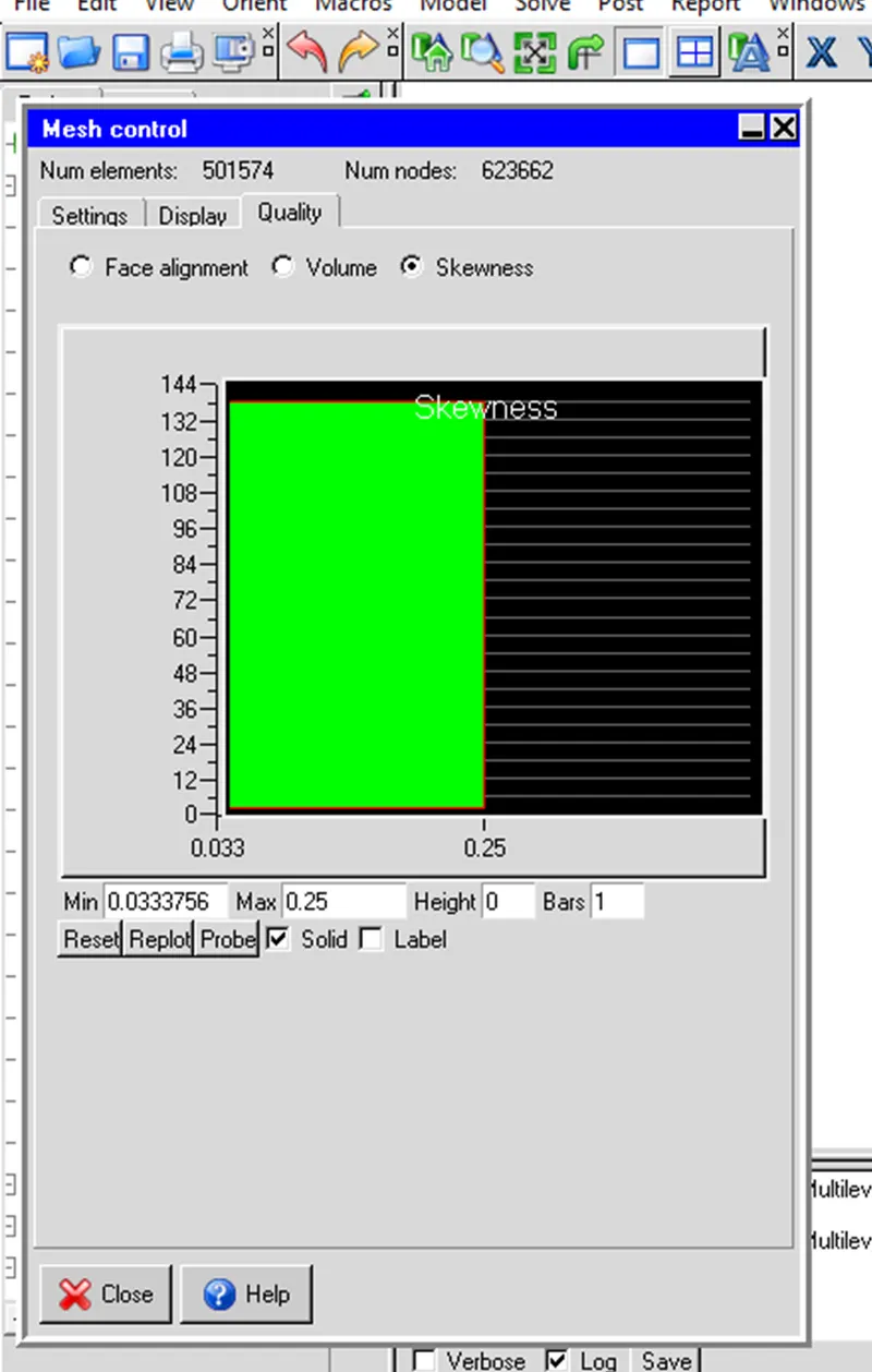
The above skewness plot shows, there are still 132 bad-quality elements, which can be further resolved to get an even better result.
Solver Set Up:
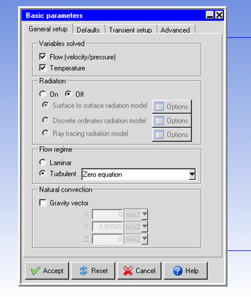
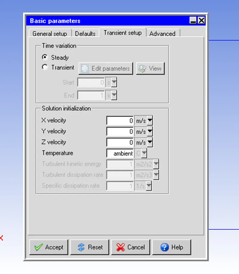
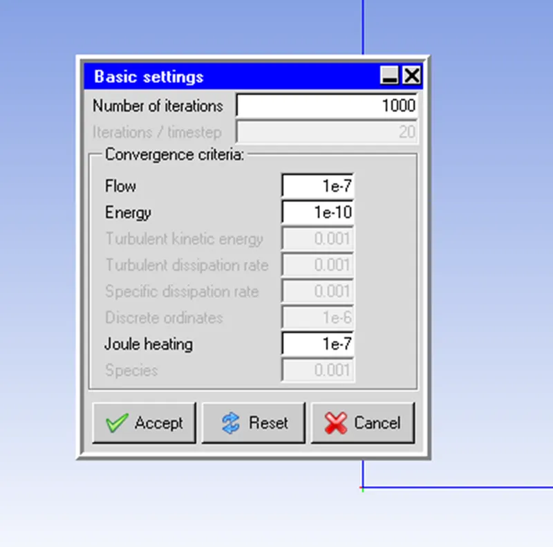
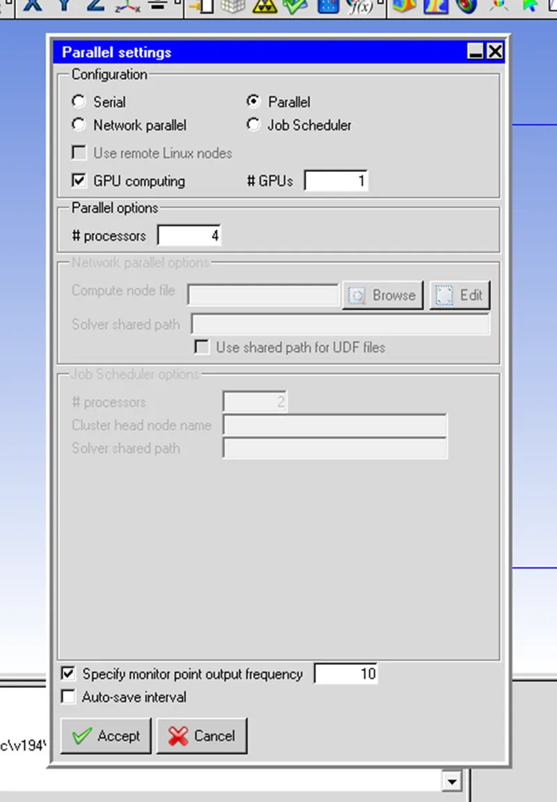
The model is to be solved for the flow and temperature variables, Radiation is kept off, and the flow regime is kept turbulent, the number of iterations is set to 1000, precision is set to double, and convergence criteria for flow: 1e-7, Energy: 1e-10, and for Joule heating: 1e-7 are set and other settings are kept as default. Fan type is set to internal, flow direction: Normal (negative), and flow type is set to non-linear.
Solution Residuals:
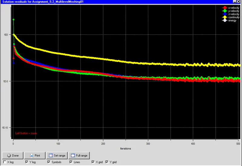
Solution residual plots show there is very little variation in variables as the steady state is reached after 300 iterations. We can observe how the solution converses with the increasing number of iterations.
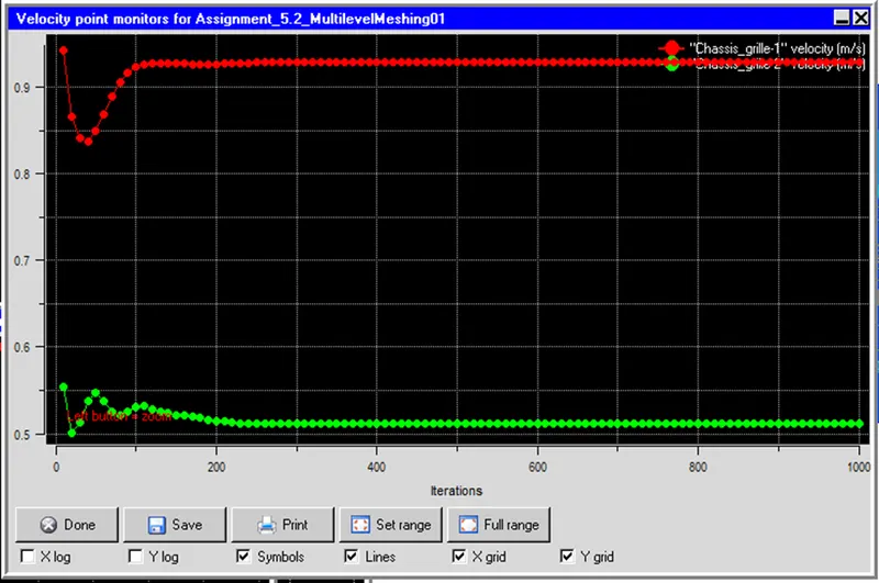
Monitor Plots:
Monitors points are set up at chassis_grille.1 and Chassis_grille.2 which shows how velocity is varying with the number of iterations. It shows velocity becomes steady after 300 iterations for both locations.
Results:
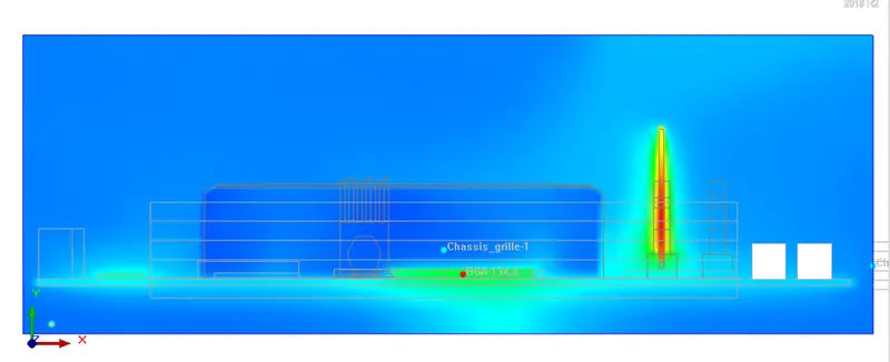
Z plane through Center
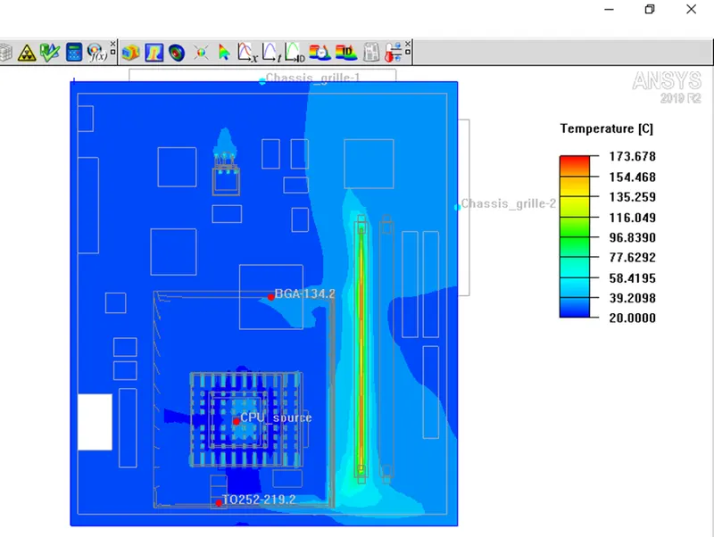
Y Plane through Center
X Plane through Center
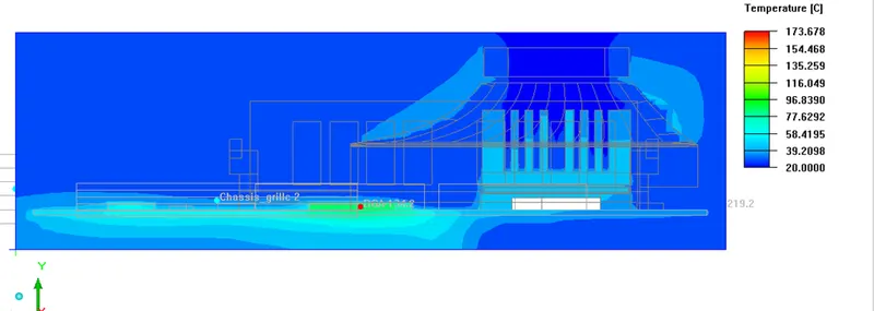
From the above X, Y, and Z cut planes contour plots passing through the center of the cabinet show how the thermal boundary layer is formed, and how heat is dissipating from hot bodies to cold bodies. Most portion of the cabinet is at ambient temperature.
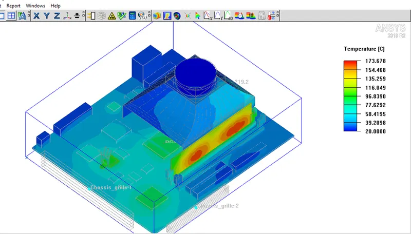
Object Face Plot
From the object face plot, the maximum temperature reached is around 173 degrees Celsius. Heat generators gained the maximum temperature, so their nearby objects were relatively at a higher temperature than the cabinet temperature.
X Plane through Center:
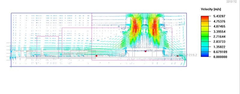
Y Plane through Center:
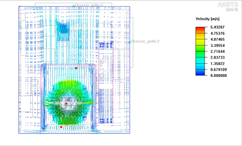
Z Plane through Center:
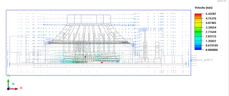
Cut plane velocity vector plots for X, Y, and Z planes passing through the center of the cabinet show how air recirculation is taking place, air speed is maximum when it passes through the fan. The maximum speed achieved is around 5.4 m/s. It shows how air takes heat from hot bodies, and gets distributed.
Conclusion:
The given model is successfully loaded to the Ansys ICEPAK, and Physical and Numerical settings are set to solve flow and temperature variables.
Cut plane contour plots and Object face contour plots are plotted for Temperature and Velocity variables.
The maximum temperature is found to be around 173 on heat-generating bodies and the maximum velocity is found to be around 5 m/s at the fan location. These plots show how thermal and fluid boundary layers are formed and how fluid is recirculating in the cabinet.