Week 11 - Simulation of Flow through a pipe in OpenFoam
SIMULATION OF FLOW THROUGH A PIPE IN OPEN FOAM
AIM:
- To simulate an axis-symmetric flow by applying the wedge boundary condition. The flow is laminar and flows through a constant cross-section pipe at an inlet Reynolds’s number of 2100.
- To validate the simulation results with the Hagen-Poiseuille’s equations for the fully developed flow.
- Also to write code in MATLAB to automate the generation of blockMeshDict file. The code will take inputs like pipe length, diameter, wedge angle, etc and output a fully functional blockMeshDict file.
THEORY:
Introduction to Internal Flow:
Liquids or gas flow through pipes or ducts is commonly used in heating and cooling applications and fluid distribution networks. The fluid in such applications is usually forced to flow by a fan or pump through a flow section. The terms pipe, duct, and conduit are usually used interchangeably for flow sections. In general, flow sections of the circular cross-section are referred to as pipes (especially when the fluid is a liquid) and flow sections of the non-circular cross-section as ducts (especially when the fluid is a gas). Small diameter pipes are usually referred to as tubes.
The fluid velocity in a pipe changes from zero at the wall because of the no-slip condition to a maximum at the pipe center. In fluid flow, it is convenient to work with an average velocity of V_avg , which remains constant in incompressible flow when the cross-sectional area of the pipe is constant.
Also, the friction between the fluid particles in a pipe does cause a slight rise in fluid temperature as a result of the mechanical energy being converted to sensible thermal energy. But this temperature rise is due to frictional heating is usually too small to warrant any consideration in calculations and thus is disregarded.
Laminar Flow and Turbulent Flow:
Laminar flow or streamline flow in pipes occurs when a fluid flows in parallel layers, with no disruption between layers. At low velocities, the fluid tends to flow without lateral mixing, and adjacent layers slide past one another like playing cards. There are no cross-currents perpendicular to the direction of flow, nor eddies or swirls of fluids. In laminar flow, the motion of the particles of the fluid is very orderly with all particles moving in straight lines parallel to the pipe walls.
Turbulent flow is a flow regime characterized by chaotic property changes. This includes rapid variation of pressure and flow velocity in space and time. In contrast to laminar flow, the fluid no longer travels in layers, and mixing across the tube is highly efficient. Flows at Reynolds numbers larger than 4000 are typically turbulent, while those at low Reynolds numbers below 2300, usually remain laminar. Flow in the range of Reynolds numbers 2300 to 4000 are known as transition.
Reynolds Number:
The transition from laminar to turbulent flow depends on the geometry, surface toughness, flow velocity, surface temperature, and type of fluid, among other things. After exhaustive experiments in the 1880s, Osborne Reynolds discovered that the flow regime depends mainly on the ratio of inertial forces to viscous forces in the fluid. This ratio is called the Reynolds number and is expressed for internal flow in a circular pipe as
`R_e = (V_(avg)*L)/nu=(V_(avg)*L*rho)/mu`
where `V_(avg)`= average flow velocity in m/s
`L`= charsteritic length of the geometry in m
`nu=mu/rho`= kinematic viscocity in m^2/s
The Entrance Length or Hydrodynamic Length:
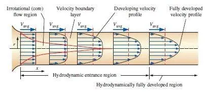
Consider a fluid entering a circular pipe at a uniform velocity. Because of the no-slip condition, the fluid particles in the layer in contact with the wall of the pipe come to a complete stop. This layer also causes the fluid particles in the adjacent layers to slow down gradually as result of friction. To make up for this velocity reduction, the velocity of the fluid at the midsection of the pipe has to increase to the mass flow rate through the pipe constant. As a result, a velocity gradient develops along the pipe.
The region of the flow in which the effects of the viscous shearing forces caused by fluid viscosity are felt is called the velocity boundary layer or just the boundary layer. The hypothetical boundary surface divides the flow in a pipe into two regions: the boundary layer region, in which the viscous effects and the velocity changes are significant, and the irrotational flow region, in which the frictional effects are negligible and the velocity remains essentially constant in the radical direction.
The thickness of this boundary layer increases in the flow direction until the boundary layer reaches the pipe center and thus fills the entire pipe and the velocity becomes fully developed a little farther downstream. The region from the pipe inlet to the point at which the velocity profile is fully developed is called the hydrodynamic entrance region, and the length of this region is called the hydrodynamic entry length L_h. Flow in the entrance region is called hydrodynamically developing flow since this is the region where the velocity profile develops. The region beyond the entrance region in which the velocity profile is fully developed and remains unchanged is called the hydrodynamically fully developed region. The flow is said to be fully developed when the normalized temperature profile remains unchanged as well.
Entry Length:
The hydrodynamic entry length is usually taken to be the distance from the pipe entrance to where the wall shear stress reaches within about 2 percent of the fully developed value. In laminar flow, the non-dimensional hydrodynamic entry length is given approximately as
`L_h=0.05*R_e*D`
Laminar Flow through Pipe:
Consider the steady, laminar, incompressible flow of fluid with constant properties in the fuly developed region of straight circular pipe. The momentum equation obtained by applying a momentum balance to a differential volume element, and also the velocity profile is obtained by solving it. Then it is used to obtain a relation for the friction factor. An important aspect of the analysis here is that it is one of the few available for viscous flow.
In fully developed laminar flow, each fluid particle moves at a constant axial velocity along a streamline and the velocity profile u(r) remains unchanged in the flow direction. There is no motion in the radial direction, and thus the velocity component in the direction normal to the pipe axis is everywhere zero. There is no acceleration since the flow is steady and fully developed.
The velocity profile is fully developed laminar flow in a pipe is parabolic with a maximum at the centerline and a minimum at the pipe wall and is given by the equation as a function of radial distance from the centre.
`u(r)=2V_(avg)(1-r^2/R^2)`
The pressure drop due to viscous effects over the length of the pipe is shown below
`DeltaP=P_1-P_2=( 8muLV_(avg))/R^2`
MATLAB PROGRAM:
%Creating the blockMeshDict file

clear all
close all
clc

%Inputs

%angle of wedge
theta= 3 ;

%Reynolds number for laminar flow
Re= 2100;

%Diameter of the pipe
D=0.02;
R=D/2;

%Length of the pipe
L=2.5;

%dynamic vsicocity
mu= 8.9e-4;

%Density of water
rho=1000;

%kinematic viscocity
nu= mu/rho;

%Number of grids along x,y and z directions
nx= 50;
ny=1;
nz= 100;

% Calculation of properties

%hydrodynamic length
Le=0.05*Re*D ;

%Average velocity
V_avg = (Re*mu)/(rho*D);

%Maximum Velocity
V_max=2*V_avg;

%Pressure difference
delta_P= (8*mu*L*V_avg)/(R^2);
kinematic_p= delta_P/rho;

%Wall shear stress
tau= (delta_P*D)/(4*L);


% Vertices of wedge
v0=[0,0,0];
v1=[0,R*cosd(theta/2),-R*sind(theta/2)];
v2=[0,R*cosd(theta/2), R*sind(theta/2)];
v3=[L,0,0];
v4=[L,R*cosd(theta/2),-R*sind(theta/2)];
v5=[L,R*cosd(theta/2), R*sind(theta/2)];

%texts of the header
text1='/*--------------------------------*- C++ -*--------------------------------*\';
text2='=========                |';
text3='\\      /  F ield        |  OpenFOAM: The Open Source CFD Toolbox';
text4=' \\    /   O peration    |  Website:  https://openfoam.org';
text5='  \\  /    A nd          |  Version:  8';
text6='   \\/     M anipulation |';
text7='\*--------------------------------*- C++ -*--------------------------------*/';

%Creating File
f1=fopen('blockMeshDict.txt','w');

%writing the blockMeshDict file
fprintf(f1,'%s\n',text1);
fprintf(f1,'%s\n',text2);
fprintf(f1,'%s\n',text3);
fprintf(f1,'%s\n',text4);
fprintf(f1,'%s\n',text5);
fprintf(f1,'%s\n',text6);
fprintf(f1,'%s\n',text7);

fprintf(f1,'FoamFile \n{\n');
fprintf(f1,'%16s %9s\n','version','2.0;');
fprintf(f1,'%15s %12s\n','format','ascii;');
fprintf(f1,'%14s %18s\n','class','dictionary;');
fprintf(f1,'%15s %20s\n','object','blockMeshDict;');
fprintf(f1,'%2s\n','}');

fprintf(f1,'%2s\n\n','//* * * * * * * * * * * * * * * * * * * * * * * * * * * * * * * * * * *//');
fprintf(f1,'%2s\n\n','convertToMeters 1;');
fprintf(f1,'vertices \n(\n');
fprintf(f1,'(%f %f %f)\n',v0);
fprintf(f1,'(%f %f %f)\n',v1);
fprintf(f1,'(%f %f %f)\n',v2);
fprintf(f1,'(%f %f %f)\n',v3);
fprintf(f1,'(%f %f %f)\n',v4);
fprintf(f1,'(%f %f %f)\n',v5);
fprintf(f1,'%2s\n\n',');');

fprintf(f1,'blocks\n(\n');
fprintf(f1,'hex(0 1 2 0 3 4 5 3) (%f %f %f) %s (%f %f %f)\n);\n\n',nx,ny,nz,'simpleGrading',0.1,1,1);
fprintf(f1,'edges \n(\n');
fprintf(f1,'%s 2 1 (%f %f %f)\n','arc',0,0.01,0);
fprintf(f1,'%s 4 5 (%f %f %f)\n','arc',2.5,0.01,0);
fprintf(f1,');\n\n');
fprintf(f1,'boundary\n(\n');
fprintf(f1,'%8s\n %s\n','axis','{');
fprintf(f1,'%12s %s\n %6s\n %4s\n %14s\n %6s\n %s\n\n','type empty',';','faces','(','(0 3 3 0)',');','}');
fprintf(f1,'%8s\n %s\n %14s %s\n %9s\n %2s\n %14s\n %4s\n %s\n\n','inlet','{','type patch',';','faces','(','(0 1 2 0)',');','}');
fprintf(f1,'%8s\n %s\n %14s %s\n %9s\n %2s\n %14s\n %4s\n %s\n\n','wall','{','type wall',';','faces','(','(2 5 4 1)',');','}');
fprintf(f1,'%8s\n %s\n %14s %s\n %9s\n %2s\n %14s\n %4s\n %s\n\n','outlet','{','type patch',';','faces','(','(3 4 5 3)',');','}');
fprintf(f1,'%8s\n %s\n %14s %s\n %9s\n %2s\n %14s\n %4s\n %s\n\n','front','{','type wedge',';','faces','(','(0 3 5 2)',');','}');
fprintf(f1,'%8s\n %s\n %14s %s\n %9s\n %2s\n %14s\n %4s\n %s\n\n','back','{','type wedge',';','faces','(','(0 1 4 3)',');','}');
fprintf(f1,'%s\n\n %s\n %s\n %s\n\n',');','mergePatchPairs','(',');');
fprintf(f1,'//****************************************************************//');

fclose(f1);
OPENFOAM PROGRAM:
BlockMeshDict
/*--------------------------------*- C++ -*--------------------------------*\
=========                |
\\      /  F ield        |  OpenFOAM: The Open Source CFD Toolbox
 \\    /   O peration    |  Website:  https://openfoam.org
  \\  /    A nd          |  Version:  8
   \\/     M anipulation |
\*--------------------------------*- C++ -*--------------------------------*/
FoamFile
{
         version      2.0;
         format       ascii;
         class        dictionary;
         object       blockMeshDict;
 }
//* * * * * * * * * * * * * * * * * * * * * * * * * * * * * * * * * * *//

convertToMeters 1;

vertices
(
    (0 0 0)
    (0 0.009997 -0.000262)
    (0 0.009997 0.000262)
    (2.5 0 0)
    (2.5 0.009997 -0.000262)
    (2.5 0.009997 0.000262)
);

blocks
(
       hex (0 1 2 0 3 4 5 3) (50 1 100) simpleGrading (0.1 1 1)
);

edges
(
    arc 2 1 (0 0.1 0)
    arc 4 5 (2.5 0.1 0)
);

boundary
(

    axis
 {
     type empty ;
     faces
    (
          (0 3 3 0)
     );
 }

   inlet
 {
     type patch ;
     faces
  (
          (0 1 2 0)
   );
 }

    wall
 {
      type wall ;
      faces
  (
          (2 5 4 1)
   );
 }

   outlet
 {
     type patch ;
     faces
  (
          (3 4 5 3)
   );
 }

   front
 {
     type wedge ;
     faces
  (
      (0 3 5 2)
   );
 }

    back
 {
     type wedge ;
     faces
  (
      (0 1 4 3)
   );
 }

);

 mergePatchPairs
 (
 );

//************************************************************************//
ControlDict
/*--------------------------------*- C++ -*----------------------------------*\
  =========                 |
  \\      /  F ield         | OpenFOAM: The Open Source CFD Toolbox
   \\    /   O peration     | Website:  https://openfoam.org
    \\  /    A nd           | Version:  8
     \\/     M anipulation  |
\*---------------------------------------------------------------------------*/
FoamFile
{
    version     2.0;
    format      ascii;
    class       dictionary;
    location    "system";
    object      controlDict;
}
// * * * * * * * * * * * * * * * * * * * * * * * * * * * * * * * * * * * * * //

application     icoFoam;

startFrom       startTime;

startTime       0;

stopAt          endTime;

endTime         30;

deltaT          1e-2;

writeControl    timeStep;

writeInterval   20;

purgeWrite      0;

writeFormat     ascii;

writePrecision  6;

writeCompression off;

timeFormat      general;

timePrecision   6;

runTimeModifiable true;


// ************************************************************************* //
Transport Properties
/*--------------------------------*- C++ -*----------------------------------*\
  =========                 |
  \\      /  F ield         | OpenFOAM: The Open Source CFD Toolbox
   \\    /   O peration     | Website:  https://openfoam.org
    \\  /    A nd           | Version:  8
     \\/     M anipulation  |
\*---------------------------------------------------------------------------*/
FoamFile
{
    version     2.0;
    format      ascii;
    class       dictionary;
    location    "constant";
    object      transportProperties;
}
// * * * * * * * * * * * * * * * * * * * * * * * * * * * * * * * * * * * * * //

nu              [0 2 -1 0 0 0 0] 8.9e-7;


// ************************************************************************* //
Pressure
/*--------------------------------*- C++ -*----------------------------------*\
  =========                 |
  \\      /  F ield         | OpenFOAM: The Open Source CFD Toolbox
   \\    /   O peration     | Website:  https://openfoam.org
    \\  /    A nd           | Version:  8
     \\/     M anipulation  |
\*---------------------------------------------------------------------------*/
FoamFile
{
    version     2.0;
    format      ascii;
    class       volScalarField;
    object      p;
}
// * * * * * * * * * * * * * * * * * * * * * * * * * * * * * * * * * * * * * //

dimensions      [0 2 -2 0 0 0 0];

internalField   uniform 0;

boundaryField
{
    axis
    {
        type            empty;
    }

    inlet
    {
        type            zeroGradient;

    }

    wall
    {
        type            zeroGradient;

    }

    outlet
    {
        type            fixedValue;
        value           uniform 0.0166;
    }

    front
    {
        type            wedge;

    }

    back
    {
        type            wedge;

    }

}

// ************************************************************************* //
Velocity
/*--------------------------------*- C++ -*----------------------------------*\
  =========                 |
  \\      /  F ield         | OpenFOAM: The Open Source CFD Toolbox
   \\    /   O peration     | Website:  https://openfoam.org
    \\  /    A nd           | Version:  8
     \\/     M anipulation  |
\*---------------------------------------------------------------------------*/
FoamFile
{
    version     2.0;
    format      ascii;
    class       volVectorField;
    object      U;
}
// * * * * * * * * * * * * * * * * * * * * * * * * * * * * * * * * * * * * * //

dimensions      [0 1 -1 0 0 0 0];

internalField   uniform (0 0 0);

boundaryField
{
    axis
    {
        type            empty;
    }

    inlet
    {
        type            fixedValue;
        value           uniform (0.0935 0 0);
    }

    outlet
    {
        type            zeroGradient;
    }

    wall
    {
        type            noSlip;

    }

    front
    {
        type            wedge;
    }

    back
    {
        type            wedge;
    }

}

// ************************************************************************* //
Once the above file are set, blockmesh command is used to generate mesh. Once the blockmesh command run sucessfully type icoFoam in the command window so that the prgram run for given amount of time using icoFoam solver. After the program run a post-processing tool is used to viw the result which is paraview . This paraview can be opened using paraFoam command.
OUTPUT :
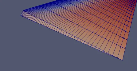
Mesh created on wedge with angle of 3 degrees :
Velocity Profile:
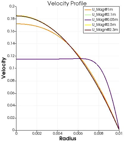
The velocity profiles above are plotted at entry 0.05m and at the midway 1m and at hydrodynamic length 2.1m and thereafter at 2.3 and 2.5 in order to show that the velocity profile doesnt change much after hydrodynamic length. From the figure we can see that the velocity profile at 2.1m almost coincides with velocity prfofile at 2.3m and 2.5m. Also , from analytical formula we got that the max velocity as 0.1869 whereas the numerical result is 0.1840 . The error occured from the results is 1.5%.
Pressure Profile:
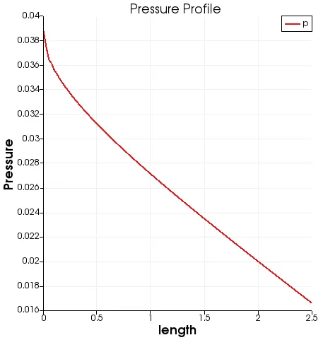
From the baove figure we can say that the pressure decreased along the length of the pipe and the numerical result of pressure difference obtained is 0.0164 and the analytical value was 0.0169. Error percentage is 1.7%
Shear Stress :
In this program shear stress cannot be plotted directly as velocity . There are few steps to be taken to calculate the value of shear stress and plot the value .
1. Open calculator tool and calculate the magnitude of u and name th result array is mag_u .
2. Later open the gradinet of unstructured dataset tool and caluclate the gradient value of u and name the array as grad_u
3. Now open a new calculator and name the result array as tau and calulate the value of tau by multiplying the grad_ with the value of mu which is 8.9e-4 . This will result in creation of tau term
4. now use the plot of line tool and plot the shear stress along the radius of pipe at hydrodynamic length @2.1m
Shear stress is calculated using the formula
`tau = mu*((du)/(dy))`
where
`tau`= Wall shear stress
`mu`= dynamic viscocity
`(du)/dy=`velocity gradient
Shear stress profile :
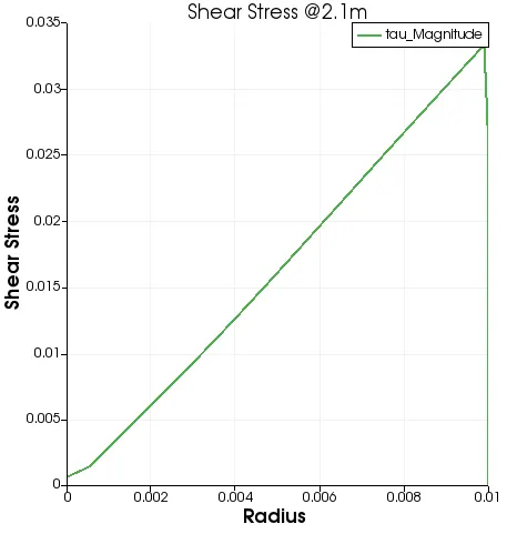
From the above graph we can say that the value of shear stress numerically is equal to 0.0332 whereas the analytical value is 0.0333 the erro percentage is almost negligible.
CONCLUSION:
1. The hydrodynamic length of 2.1m is validated in the simulation result and was also explanied with help of velocity profile variation along the length.
2. The maximum velocity of fully developed laminar flow is also validated using the simulation result along with the graphs and the erro was fund to be around 1.5 percent which is under standard range.
3. The Shear stress is post-processed and was validated using the simulation result .The value of wall-shear is compared to the analytical values and the errror was found to be 0.3%
4. The pressure difference along the length of pipe is found and was validated with analytical result and obtained an error os around 1.7%
5. BlockMeshDict file is written using matlab and was used in openFoam for the simulation.