Week 11 - Simulation of Flow through a pipe in OpenFoam
AIM :
The Objectives of the project are :-
(i) Calculation of flow variables
(ii) To Generate BlockMeshDict Using the wedge Boundry condition
(iii) The BlockMesh file should be genrated using the Matlab code ]
(iv) To stimulate the Laminar flow in the Pipe Using the Icofoam solver
(v) To Post process the result and plot the required plots using para view
Assumptions made :
Steady flow , incompressible and laminar flow
Two dimensional flow
Constant fluid properties (viscosity,Density etc)
Laminar Flow through pipe :
In pipes (or tubes), laminar flow or streamline flow occurs when a fluid flows in parallel layers with no interruption between them. The fluid tends to flow without lateral mixing at low velocities, and neighbouring layers slide past each other like playing cards. There are no eddies or swirls of fluids, nor are there cross-currents perpendicular to the flow direction. The motion of the fluid particles is exceedingly ordered in laminar flow, with all particles travelling in straight lines parallel to the pipe walls.

Fig 1 : Laminar FLow
Turbulent Flow through pipe :
Turbulent flow is characterised by erratic property changes in the flow. This includes rapid changes in pressure and flow velocity throughout time and place. Unlike laminar flow, the fluid does not travel in layers, and mixing across the tube is extremely efficient. Flows with Reynolds numbers greater than 4000 are usually (but not always) turbulent, and those with Reynolds values less than 2300 are usually laminar. Transitional flow is defined as flow with Reynolds numbers ranging from 2300 to 4000.

Fig 2 : Turbulent Flow
Reynolds Number :
The geometry, surface roughness, flow velocity, surface temperature, and fluid type all play a role in the transition from laminar to turbulent flow. Osborne Reynolds found in the 1880s that the flow regime is mostly determined by the ratio of inertial forces to viscous forces in the fluid. For internal flow in a circular pipe, this ratio is known as the Reynolds number, and it is stated as:
Re = Inertial forces / Viscous forces
`Re = (V_(avg)*D)/v`
= Inertial forces / Viscous forces
= `(rho*V_(avg)*D)/mu`
where ,
v = viscous force
rho = Density
D = Diameter of the Pipe
`mu =` Viscosity
The Reynolds number is a one-dimensional quantity. Kinematic viscosity is measured in m2/s and is also known as viscous diffusivity or momentum diffusivity.The inertial forces, which are related to the fluid density and the square of the fluid velocity, are large relative to the viscous forces at large Reynolds numbers, and so the viscous forces cannot prevent the fluid from fluctuating randomly and rapidly. The viscous forces are substantial enough to control these oscillations and keep the fluid “in line” at small or moderate Reynolds numbers. As a result, in the first scenario, the flow is turbulent, whereas in the second, it is laminar.
Hydrodynamic Entry Length :
The velocity boundary layer, or simply the boundary layer, is the region of the flow where the effects of viscous shearing forces induced by fluid viscosity are felt. The boundary layer zone, where viscous effects and velocity changes are considerable, and the irrotational (core) flow zone, where frictional effects are minor and the velocity remains practically constant in the radial direction, are separated by the hypothetical boundary surface.The thickness of this boundary layer expands in the flow direction until it reaches the pipe centre, filling the entire pipe, and the velocity develops fully a little further downstream. The hydrodynamic entrance region is defined as the area between the pipe inlet and the point at which the velocity profile is fully developed, and the length of this region is defined as the hydrodynamic entry length `L_h`.
Because this is where the velocity profile develops, flow in the entrance zone is referred to as hydrodynamically developing flow. The hydrodynamically fully developed region is the area beyond the entrance region where the velocity profile is entirely developed and remains unchanged.
Because this is where the velocity profile develops, flow in the entrance zone is referred to as hydrodynamically developing flow. The hydrodynamically fully developed region is the area beyond the entrance region where the velocity profile is entirely developed and remains unchanged. When the normalised temperature profile remains unchanged, the flow is said to be completely developed. When the fluid in the pipe is not heated or cooled, hydrodynamically fully developed flow is similar to fully developed flow since the fluid temperature remains virtually constant throughout. Due to eddy motion and more strong mixing in the radial direction, the velocity profile in the fully formed region is parabolic in laminar flow and significantly flatter (or fuller) in turbulent flow. When the flow is fully developed, the time-averaged velocity profile remains unchanged, and thus:
`(partialu(r,x))/(partialx) = 0`
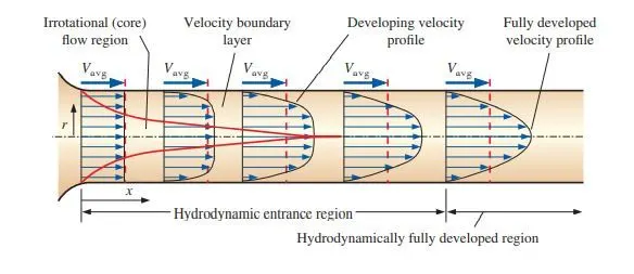
Fig 3 : Hydrodynamically Fully developed region
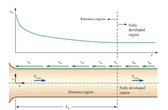
Fig 4 : The variation of wall shear stress in the flow direction
Hagen Poiseuille's Law :
In Non-ideal fluid dynamics , Hagen-poiseuille equation is a physical law that gives pressure drop in an incompressible and newtonian fluid in a laminar flow through a long cylinder pipe of constant cross section.
Formulas :
`Re = (rho*V_(avg)*D)/mu`
`V_(avg) = (Re*mu)/(rho*D)`
`V_(max) = 2*V_(avg)`
`triangleP` (Pressure difference) = `(8*mu*L.V_(avg))/(r^2)`
`triangleP_k`(Kinematic presure difference) = `(triangle P )/rho`
shear stress(`tau`) = `(2*mu*V_max *R )/r^2`
Proccedure :
In this project to stimulate a flow through the pipe we are using an axi-symetric model. The axis-symetric model of the pipe is as shown below.
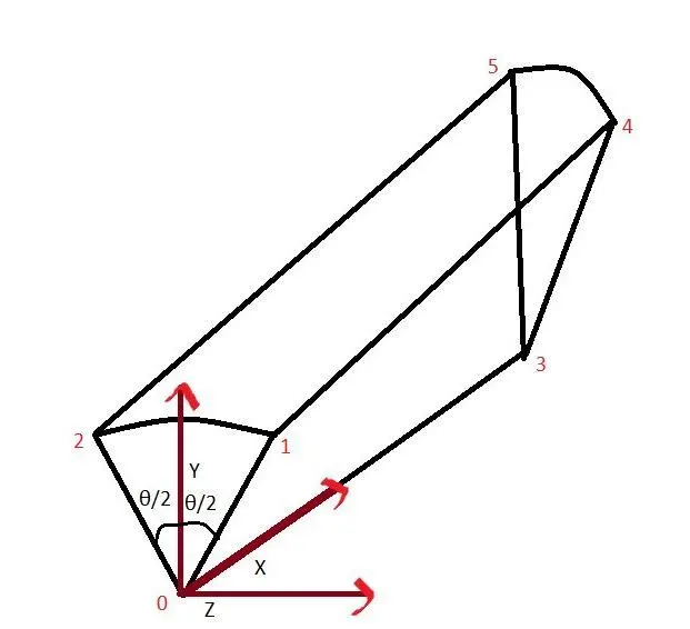
Fig 5 : Axi-symetric pipe
The coordinates of the Pipe are as follows :
(0, 0, 0 ) `->` 0
(0, `r*cos((theta)/2)`, `r*sin((theta)/2)` ) `->` 1
(0, `r*cos((theta)/2)`, `-r*sin((theta)/2)` ) `->` 2
(`L_p`, 0, 0 ) `->` 3
(`L_p`, `r*cos((theta)/2)`, `r*sin((theta)/2)` ) `->` 4
(`L_p`, `r*cos((theta)/2)`, `-r*sin((theta)/2)`) `->` 5
L_p = Hydrodynamic_Length + 0.7
L_p = Total length of the pipe
To stimulate the flow through a pipe using IcoFoam we have to follow these steps :
1. Create a matlab code to genrate a blockmeshDict file
2. The Boundry conditions like velocity pressure for the stimulation is set in the Initial condition folder
3. The blockmesh command is initiated and the mesh geometry is created in the constant folder
4. The stimulation is achieved using the IcoFoam solver
Matlab code :
close all
clear all
clc
%% Inputs
% The Reynolds Number
Re = 2100
% The Diameter of the Pipe
D = input('Dia in mm : ');

% The Entry length of the Pipe
L = 0.06 * Re * D
L_p = L+ 0.7

% Radius of the Pipe
r = D/2
% Angle of wedge
teta = input('Enter value less than 5 Degrees : ')

% Dynamic viscosity
mu = 0.89e-3
% Density
rho  = 997

%% Haigen Poisle Flow Equation
v_avg = (Re*mu)/(rho*D)
v_max = 2*(v_avg)
del_p = (8*mu*L_p*v_avg)/(r^2)
ke_p = del_p/rho

%% Calculating the shear stress
R = linspace(0,r,1000);
for i = 1:length(R)
    tou(i) = 2*mu*v_max*(abs(R(i)))/r^2;
end
plot(R,tou)
xlabel('Radius')
ylabel('Shear stress')
grid on
legend('shear stress')

%% To create Mesh
% Vertices of the coordinates
v0 = [0 0 0]
v1 = [0 r*cosd(teta/2) r*sind(teta/2)]
v2 = [0 r*cosd(teta/2) -r*sind(teta/2)];
v3 = [L_p 0 0]
v4 = [L_p r*cosd(teta/2) r*sind(teta/2)]
v5 = [L_p r*cosd(teta/2) -r*sind(teta/2)]

%% Header Defination
h_1='/*--------------------------------*- C++ -*----------------------------------*\';
h_2='  =========                 |                                                    ';
h_3='  \\      /  F ield         | OpenFOAM: The Open Source CFD Toolbox            ';
h_4='   \\    /   O peration     | Website:  https://openfoam.org                   ';
h_5='    \\  /    A nd           | Version:  8                                      ';
h_6='     \\/     M anipulation  |                                                  ';
h_7='\*---------------------------------------------------------------------------*/';
h_8='FoamFile';
h_9='{';
h_10='  version     2.0;' ;
h_11='  format      ascii;';
h_12='  class       dictionary;';
h_13='  object      blockMeshDict;';
h_14='}';
h_15='// * * * * * * * * * * * * * * * * * * * * * * * * * * * * * * * * * * * * * //';

conv ='convertToMeters 1;';

f1 = fopen('blockMeshDict','wt') %% To open the text folder
%% Creating the Header files and comments
fprintf(f1,'%s\n',h_1);
fprintf(f1, '%s\n', h_2);
fprintf(f1, '%s\n', h_3);
fprintf(f1, '%s\n', h_4);
fprintf(f1, '%s\n', h_5);
fprintf(f1, '%s\n', h_6);
fprintf(f1, '%s\n', h_7);
fprintf(f1, '%s\n', h_8);
fprintf(f1, '%s\n', h_9);
fprintf(f1, '%s\n', h_10);
fprintf(f1, '%s\n', h_11);
fprintf(f1, '%s\n', h_12);
fprintf(f1, '%s\n', h_13);
fprintf(f1, '%s\n', h_14);
fprintf(f1, '%s\n\n', h_15);

fprintf(f1, '%s\n',conv);

fprintf(f1, 'vertices\n');
fprintf(f1, '(\n');
fprintf(f1, '\t(%d %d %d)\n',v0);
fprintf(f1, '\t(%d %d %d)\n',v1);
fprintf(f1, '\t(%d %d %d)\n',v2);
fprintf(f1, '\t(%d %d %d)\n',v3);
fprintf(f1, '\t(%d %d %d)\n',v4);
fprintf(f1, '\t(%d %d %d)\n',v5);
fprintf(f1, ');\n\n');

%% Blocks Defination
fprintf(f1, 'blocks\n');
fprintf(f1, '(\n');
fprintf(f1, '\t hex (0 3 5 2 0 3 4 1)(%d %d %d)',300,30,1);
fprintf(f1, ' SimpleGrading (1 0.1 1)\n\n');
fprintf(f1, ');\n\n');
%% Edges Defination
fprintf(f1, 'edges\n');
fprintf(f1, '(\n');
fprintf(f1, '\t arc %d %d (%d %d %d)\n',1,2,0,r,0);
fprintf(f1, '\t arc %d %d (%d %d %d)\n',4,5,L_p,r,0);
fprintf(f1, ');\n\n');
%% Inlet
fprintf(f1, 'boundry\n');
fprintf(f1, '(\n');
fprintf(f1, '\t inlet \n');
fprintf(f1, '\t {\n');
fprintf(f1, '\t\t type patch;\n');
fprintf(f1, '\t\t faces \n');
fprintf(f1, '\t\t (\n');
fprintf(f1, '\t\t\t (0 1 2 0)\n');
fprintf(f1, '\t\t );\n');
fprintf(f1, '\t }\n');
%% Outlet Defination
fprintf(f1, '\t outlet \n');
fprintf(f1, '\t {\n');
fprintf(f1, '\t\t type patch;\n');
fprintf(f1, '\t\t faces \n');
fprintf(f1, '\t\t (\n');
fprintf(f1, '\t\t\t (3 5 4 3)\n');
fprintf(f1, '\t\t );\n');
fprintf(f1, '\t }\n');
%% Top
fprintf(f1, '\t top \n');
fprintf(f1, '\t {\n');
fprintf(f1, '\t\t type wall;\n');
fprintf(f1, '\t\t faces \n');
fprintf(f1, '\t\t (\n');
fprintf(f1, '\t\t\t (1 4 5 2)\n');
fprintf(f1, '\t\t );\n');
fprintf(f1, '\t }\n');
%% Front
fprintf(f1, '\t front \n');
fprintf(f1, '\t {\n');
fprintf(f1, '\t\t type wedge;\n');
fprintf(f1, '\t\t faces \n');
fprintf(f1, '\t\t (\n');
fprintf(f1, '\t\t\t (0 3 4 1)\n');
fprintf(f1, '\t\t );\n');
fprintf(f1, '\t }\n');
%% Back
fprintf(f1, '\t back \n');
fprintf(f1, '\t {\n');
fprintf(f1, '\t\t type wedge;\n');
fprintf(f1, '\t\t faces \n');
fprintf(f1, '\t\t (\n');
fprintf(f1, '\t\t\t (0 2 5 3)\n');
fprintf(f1, '\t\t );\n');
fprintf(f1, '\t }\n');
%% Axis
fprintf(f1, '\t axis \n');
fprintf(f1, '\t {\n');
fprintf(f1, '\t\t type empty;\n');
fprintf(f1, '\t\t faces \n');
fprintf(f1, '\t\t (\n');
fprintf(f1, '\t\t\t (0 3 3 0)\n');
fprintf(f1, '\t\t );\n');
fprintf(f1, '\t }\n');
fprintf(f1, '); \n\n');

fprintf(f1, 'mergePatchPairs\n');
fprintf(f1, '(\n');
fprintf(f1, ');\n');

h_17='//***********************************************************************//';
fprintf(f1, '%s\n',h_17);

fclose(f1);

%%
Fig 6 : Matlab Code
BlockMeshDict File :
/*--------------------------------*- C++ -*----------------------------------*\
  =========                 |
  \\      /  F ield         | OpenFOAM: The Open Source CFD Toolbox
   \\    /   O peration     | Website:  https://openfoam.org
    \\  /    A nd           | Version:  8
     \\/     M anipulation  |
\*---------------------------------------------------------------------------*/
FoamFile
{
    version     2.0;
    format      ascii;
    class       dictionary;
    object      blockMeshDict;
}
// * * * * * * * * * * * * * * * * * * * * * * * * * * * * * * * * * * * * * //

convertToMeters 1;

vertices
(
    // 1st Face set

    (0 0 0)             //0
    (0 1.998096e-03 8.723877e-05)          //1
    (0 1.998096e-03 -8.723877e-05)         //2
    (1.204000e+00 0 0)       //3
    (1.204000e+00 1.998096e-03 8.723877e-05)          //4
    (1.204000e+00 1.998096e-03 -8.723877e-05)        //5


);

blocks
(
    hex (0 3 5 2 0 3 4 1) (300 30 1) simpleGrading (1 0.1 1)


);

edges
(
     arc 1 2 (0 2.000000e-03 0)
     arc 4 5 (1.204000e+00 2.000000e-03 0)
);

boundary
(
    inlet
    {
        type patch;
        faces
        (
            (0 1 2 0)

        );
    }
    outlet
    {
        type patch;
        faces
        (
            (3 5 4 3)

        );
    }

    top
    {
        type wall;
        faces
        (
            (1 4 5 2)


        );
    }

    front
    {
        type wedge;
        faces
        (
            (0 3 4 1)


        );
    }

    back
    {
        type wedge;
        faces
        (
            (0 2 5 3)


        );
    }

    axis
    {
        type empty;
        faces
        (
            (0 3 3 0)


        );
    }

);

mergePatchPairs
(

);

//***********************************************************************//
Fig 7 : BlockMeshDict file
Pressure :
/*--------------------------------*- C++ -*----------------------------------*\
  =========                 |
  \\      /  F ield         | OpenFOAM: The Open Source CFD Toolbox
   \\    /   O peration     | Website:  https://openfoam.org
    \\  /    A nd           | Version:  8
     \\/     M anipulation  |
\*---------------------------------------------------------------------------*/
FoamFile
{
    version     2.0;
    format      ascii;
    class       volScalarField;
    object      p;
}
// * * * * * * * * * * * * * * * * * * * * * * * * * * * * * * * * * * * * * //

dimensions      [0 2 -2 0 0 0 0];

internalField   uniform 0;

boundaryField
{
    inlet
    {
        type            zeroGradient;
    }

    outlet
    {
        type            fixedValue;
        value           uniform 1.0073;
    }

    axis
    {
        type            empty;
    }

    top
    {
        type            zeroGradient;

    }

    front
    {
        type            wedge;

    }

    back
    {
        type            wedge;

    }
Fig 8 : Pressure (Initial boundry conditon
Velocity :
/*--------------------------------*- C++ -*----------------------------------*\
  =========                 |
  \\      /  F ield         | OpenFOAM: The Open Source CFD Toolbox
   \\    /   O peration     | Website:  https://openfoam.org
    \\  /    A nd           | Version:  8
     \\/     M anipulation  |
\*---------------------------------------------------------------------------*/
FoamFile
{
    version     2.0;
    format      ascii;
    class       volVectorField;
    object      U;
}
// * * * * * * * * * * * * * * * * * * * * * * * * * * * * * * * * * * * * * //

dimensions      [0 1 -1 0 0 0 0];

internalField   uniform (0 0 0);

boundaryField
{
    inlet
    {
        type            fixedValue;
        value           uniform (0.4686 0 0);
    }

    outlet
    {
        type            zeroGradient;

    }

    axis
    {
        type            empty;
    }

    top
    {
        type            fixedValue;
        value           uniform (0 0 0);
    }

    front
    {
        type            wedge;

    }

    back
    {
        type            wedge;

    }


}

// ************************************************************************* //
Fig 9 : Velocity (Initial condition)
Transport Properties :
/*--------------------------------*- C++ -*----------------------------------*\
  =========                 |
  \\      /  F ield         | OpenFOAM: The Open Source CFD Toolbox
   \\    /   O peration     | Website:  https://openfoam.org
    \\  /    A nd           | Version:  8
     \\/     M anipulation  |
\*---------------------------------------------------------------------------*/
FoamFile
{
    version     2.0;
    format      ascii;
    class       dictionary;
    location    "constant";
    object      transportProperties;
}
// * * * * * * * * * * * * * * * * * * * * * * * * * * * * * * * * * * * * * //

transportModel  Newtonian;

nu              [0 2 -1 0 0 0 0] 8.9256e-07;

// ************************************************************************* //
Fig 10 : Transport properties
Re =

        2100

Dia in mm : 0.004

L =

    0.5040


L_p =

    1.2040


r =

    0.0020

Enter value less than 5 Degrees : 5

teta =

     5


mu =

   8.9000e-04


rho =

   997


v_avg =

    0.4687


v_max =

    0.9373


del_p =

   1.0044e+03


ke_p =

    1.0074
Fig 11 : Matlab code output
Results And output
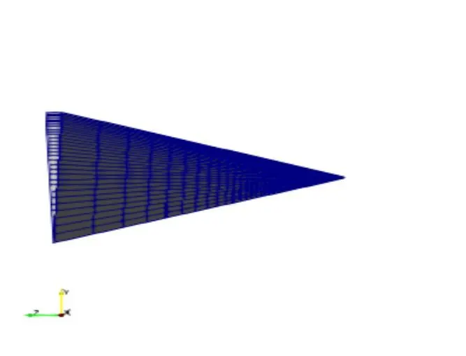
Fig 12 : Block Mesh pipe
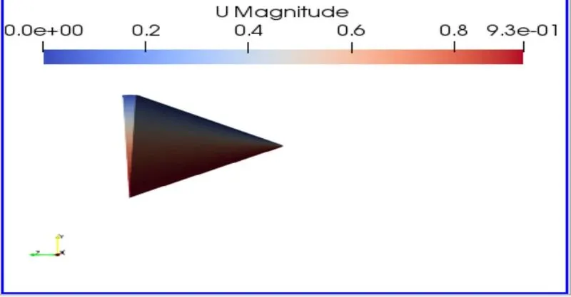
Fig 13 : velocity profile in Pipe flow
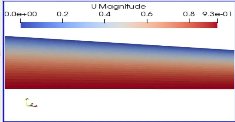
Fig 14 : Velocity profile
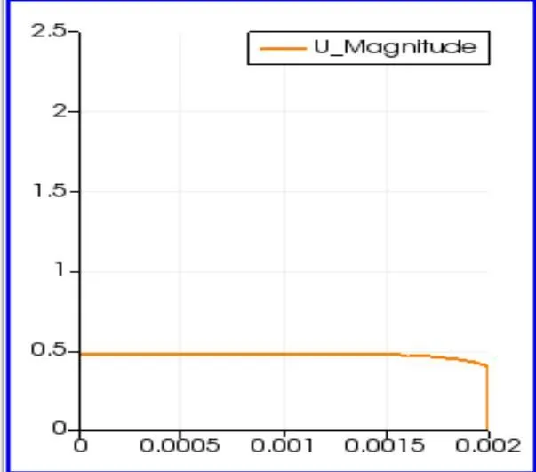
Fig 15 : Velocity profile when the Entry length 0.001 m
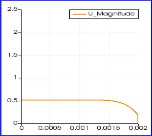
Fig 16 : Velocity profile when the Entry length 0.005 m
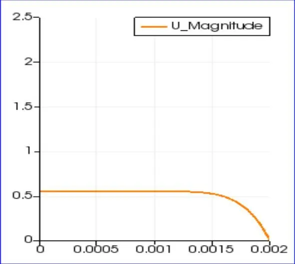
Fig 17 : Velocity profile when the Entry length is 0.009 m length
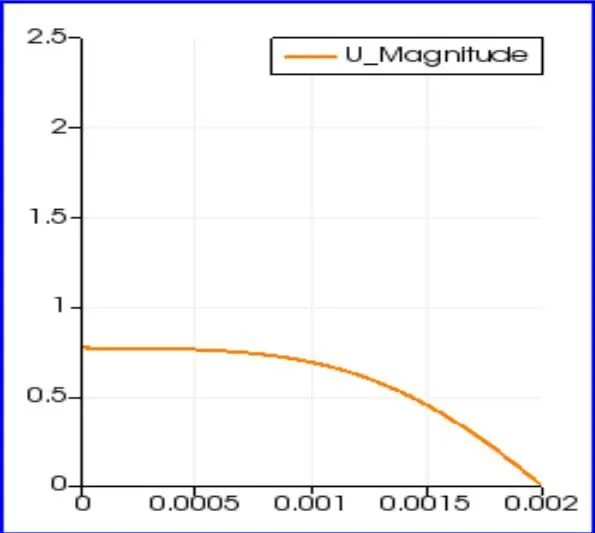
Fig 18 : Velocity profile when the Entry length is 0.1 length
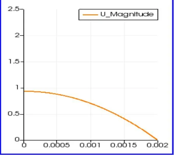
Fig 19 : Velocity profile when the Entry length is 1.1 m length
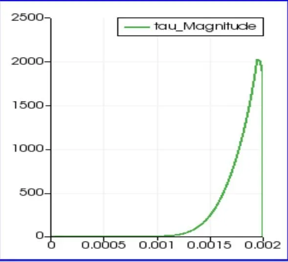
Fig 20 : shear stress profile when the Entry length of the pipe is 0.01 m
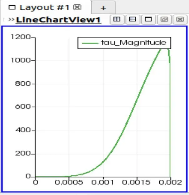
Fig 21 : shear stress profile when the Entry length of the pipe is 0.05 m length
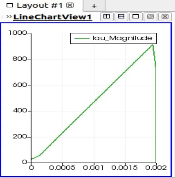
Fig 22 : shear stress profile when the Entry length of the pipe is 1m length
Results And Discussion :
From Fig 13 and Fig 14 we can say that the velocity of the fluid flowing through the pipe is minimal at the wall which is as we stated in the Initial boundry condition.
From the velocity plots from Fig 15 to Fig 19 we can see clearly that how the Fluid flow changes throughout the length of the pipe . when the length of the pipe is less than the hydrodynamic length the velocity profile is sharp as shown in fig 15 to 17.
when the velocity profile is plotted after hydrodynamic length the profile smooth and parabolic as shown in Fig 19.
The shear stress profile at the hydrodynamic length is as shown in Fig 20 , the shear stres is constant and shoots up suddenly as shown.
As the shear stress is plotted after the hydrodynamic length the plot increases gradually with respect to the radial distance of the pipe as shown in fig 22.
The radial distance in points from the stimulation is taken as an output in csv format . The Analytical solution of the stimulation is plotted using this data .
The velocity magnitude v(r) = `2*V_(avg)(1-r^2/R^2)` is calculated for the all the radial distance (`r/R`) value and a graph is plotted as shown in Fig 23 & Fig 24 .
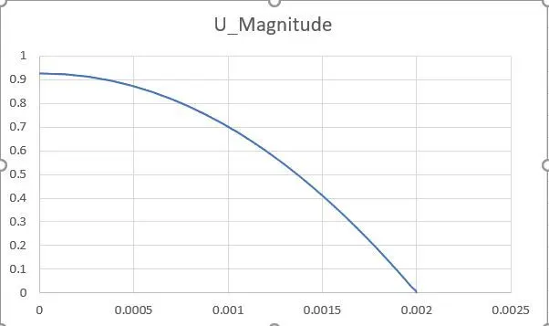
Fig 23 : The velocity profile genrated from the data exported from the stimulation
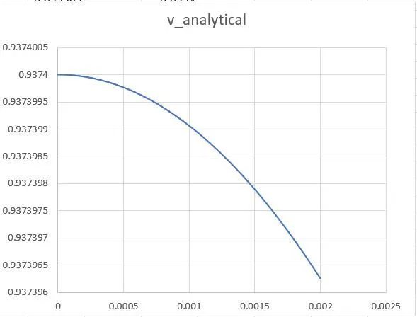
Fig 24 : V(r) vs radial distance
From the Fig 22 we can say that the graph plotted from analytical solution is same as the graph extracted from openFoam from which we can say that the stimulation is accurate and correct and results are as expected.