Week 11 - Simulation of Flow through a pipe in OpenFoam
Simulation of Flow through a pipe in OpenFoam
Aim:
in this challenge, we are going to simulate an axisymmetric flow by applying the wedge boundary condition. The flow is laminar and flows through a constant cross-section pipe. simulation results validated with the Hagen- Poiseuille's equations for the fully developed flow.
Expected Results:
- Matlab code that automates the generation of blockMeshDict file, by taking inputs like pipe length, diameter, wedge angle, etc and output a fully functional blockMeshDict file.
- Validate Hydro-dynamic length with the numerical result
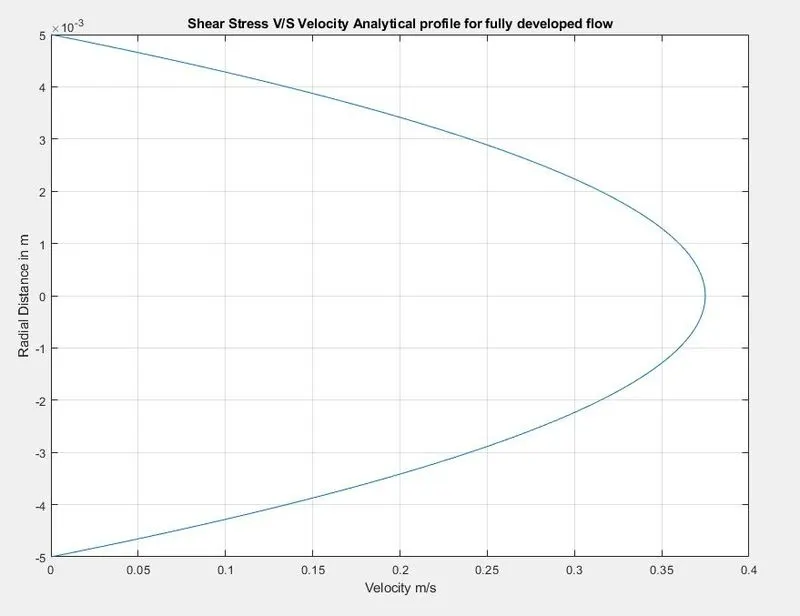
- Validate the fully developed flow velocity profile with its analytical profile
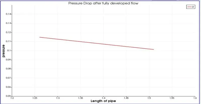
- Validate maximum velocity and pressure drop for fully developed flow
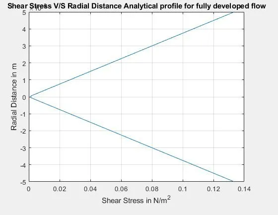
- Post-process Shear stress and validate wall shear stress for fully developed flow
Hydrodynamic entrance length:
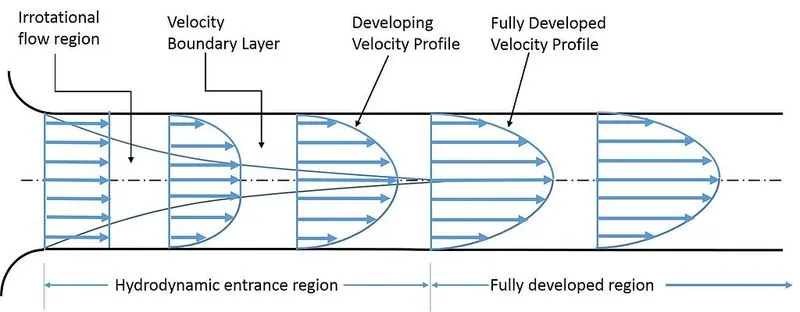
The hydrodynamic entrance region refers to the area of a pipe where fluid entering a pipe develops a velocity profile due to viscous forces propagating from the interior wall of a pipe. This region is characterized by a non-uniform flow. The fluid enters a pipe at a uniform velocity, then fluid particles in the layer in contact with the surface of the pipe come to a complete stop due to the no-slip condition. Due to viscous forces within the fluid, the layer in contact with the pipe surface resists the motion of adjacent layers and slows adjacent layers of fluid down gradually, forming a velocity profile. For the conservation of mass to hold true, the velocity of layers of the fluid in the center of the pipe increases to compensate for the reduced velocities of the layers of fluid near the pipe surface. This develops a velocity gradient across the cross-section of the pipe.
Boundary layer:
The layer in which the shearing viscous forces are significant is called the boundary layer. This boundary layer is a hypothetical concept. It divides the flow in pipe into two regions:
Boundary layer region: The region in which viscous effects and the velocity changes are significant.
The irrotational (core) flow region: The region in which viscous effects and velocity changes are negligible, also known as the inviscid core.
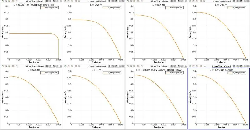
When the fluid just enters the pipe, the thickness of the boundary layer gradually increases from zero moving in the direction of fluid flow and eventually reaches the pipe center and fills the entire pipe. This region from the entrance of pipe to the point where the boundary layer covers the entire pipe is termed as the hydrodynamic entrance region and length of the pipe in this region is termed as the hydrodynamic entry length. In this region, the velocity profile develops and thus the flow is called the hydrodynamically developing flow. After this region, the velocity profile is fully developed and continues unchanged. This region is called the hydrodynamically fully developed region. But this is not the fully developed fluid flow until the normalized temperature profile also becomes constant.
In case of laminar flow, the velocity profile in the fully developed region is parabolic but in the case of turbulent flow it gets a little flatter due to vigorous mixing in radial direction and eddy motion.The velocity profile remains unchanged in the fully developed region.
`L_e /D ~~ 0.06*R_e text( for Laminar Flow)`
`L_e /D ~~ 4.4*R_e^(1/6) text( for Turbulent Flow)`
`Re <= 2300`, for a laminar flow. Under turbulent conditions it ranges from (at `Re = 4000 -10^8`).
Hagen–Poiseuille equation:
Poiseuille equation is a physical law that gives the pressure drop in an incompressible and Newtonian fluid in laminar flow flowing through a long cylindrical pipe of constant cross-section.
Pressure Drop `DeltaP = (32*mu*L.V_(avg))/D^2`
Average Velocity `V_(avg) = (R_e*mu)/(rho*D)`
Maximum Velocity `V_(max)= 2*V_(avg)`
Kinematic Pressure Drop `DeltaP_k= (DeltaP)/rho`
Velocity at 'r' `V(r) = V_(max)*(1-r^2/R^2)`
Shear stress at 'r' `tau(r) = (2*mu*V_(max)*r)/(R^2)`
Shear stress maximum at R = r
Input Data:
Diameter of pipe `D = 0.1 m`.
Renolds number `Re = 2100 text( Laminar)`.
Density of Water `rho = 997 text( kg/m3)`
Dynamic Viscosity `mu = 0.00089 text( Pa.s)`
Calculation procedure:
- Hydrodynamic entrance length `L_e = 0.06*Re*D` = 1.26 m
- Pipe length `L = L_e + 0.25` = 1.51 m
- kinematic viscosity `nu = mu/rho` = 8.92e-07
- Pipe radius `R = D/2` = 0.005 m
- Average velocity `V_(avg) = (Re*mu)/(rho*D)` = 0.187 m/s
- Maximum velocity `V_max = 2*V_(avg)`= 0.3749 m/s
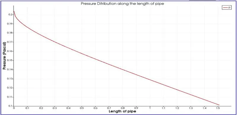
- Pressure drop `Delta_P = (32*mu*L*V_(avg))/(D^2)` =80.6178 pascal
- Kinematic pressure drop `K_P = Delta_P/rho` = 0.0809
- r = small section radius
- Velocity at various r => `V = V_max*(1-((r^2)/(R^2)))`
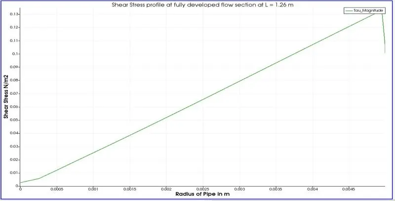
- Shear stress along cross section => `tau = (2*mu*V_max*r)/(R^2)`
Matlab program to generate blockMeshDict file using Pipe diameter, wedge angle as input. other inputs to generate Analytical solutions and plots.
% Simulation of flow through pipe project
%creating blockMeshdict file
clear all ; close all; clc

%inputs
%%
inputs  = {'Renolds number for laminar flow (Re)';'Density of working fluid (rho) kg/m^3';
           'Pipe Diameter in meters';'Wedge angle < 5 degrees';'Dynamic viscosity Pa.s'};
dlgtitle = 'Inputs & constants';
dims     = [1 50];
definput = {'2100';'997';'0.01';'3';'0.00089'};
      A  = inputdlg(inputs,dlgtitle,dims,definput);

 Re     =  str2double(A{1});                     % Renolds number for laminar flow
 rho    =  str2double(A{2});                     % Density of working fluid (rho) kg/m^3
 D      =  str2double(A{3}) ;                    % Pipe Diameter in meters
 theta  =  str2double(A{4});                     % Wedge angle < 5 degrees
 mu     =  str2double(A{5});                     % Dynamic Viscosity N/

%%
%calculations
L_e  =  0.06*Re*D; %The entrance length is the length in a tube or duct after an obstruction - until the flow velocity profile is fully developed
L    =  L_e + 0.25;   % Pipe length
K_V   = mu/rho; % kinematic viscosity
R =  D/2; %radius
V_avg    = (Re*mu)/(rho*D); %Average velocity
V_max    = 2*V_avg;  % Maximum velocity
delta_P  = (32*mu*L*V_avg)/(D^2);  % Pressure drop
delta_Pe  = (32*mu*(L-L_e)*V_avg)/(D^2);  % Pressure drop
K_P      = delta_P/rho; % Kinematic pressure drop
K_Pe      = delta_Pe/rho;
r= linspace(-0.005,0.005,100);
for i = 1:length(r)
    V(i) = V_max*(1-((r(i)^2)/(R^2)));
    Tau(i) = (2*mu*V_max*abs(r(i)))/(R^2);
end

%%
inputs   = {'Number of cells along the length of pipe';'Number of cells radially';
            'Number of cells in wedge';'Grading factor along the length of pipe';'Grading factor along radially';'Grading factor along wedge'};
dlgtitle = 'Mesh inputs';
dims     = [1 50];
definput = {'200';'50';'1';'1';'0.2';'1'};
   B     = inputdlg(inputs,dlgtitle,dims,definput);

%inputs
 nx  =  str2double(B{1});
 ny  =  str2double(B{2});
 nz  =  str2double(B{3}) ;
 Gx  =  str2double(B{4});
 Gy  =  str2double(B{5});
 Gz  =  str2double(B{6});
 %%

 % % vertices co-ordinate
  vertices = [0   0                 0;                  % point 0
              0   R*cosd(theta/2)  -R*sind(theta/2);    % point 1
              0   R*cosd(theta/2)   R*sind(theta/2);    % point 2
              L   0                 0;                  % point 3
              L   R*cosd(theta/2)  -R*sind(theta/2);    % point 4
              L   R*cosd(theta/2)   R*sind(theta/2)];   % point 5

% header lines
header = {'/*--------------------------------*- C++ -*----------------------------------*\';
          '  =========                 |';
          '  \\      /  F ield         | OpenFOAM: The Open Source CFD Toolbox';
          '   \\    /   O peration     | Website:  https://openfoam.org';
          '    \\  /    A nd           | Version:  8';
          '     \\/     M anipulation  |';
          '\*---------------------------------------------------------------------------*/';
          'FoamFile';
          '{';
          '    version     2.0;';
          '    format      ascii;';
          '    class       dictionary;';
          '    object      blockMeshDict;';
          '}';
          '// * * * * * * * * * * * * * * * * * * * * * * * * * * * * * * * * * * * * * //';};

% creating block mesh file file
     B_M_file  = fopen('blockMeshDict.txt', 'w+');
 % header
    for i = 1:15
        fprintf(B_M_file,'%s\n', string(header(i)));
    end

    fprintf(B_M_file,'\n %s \n\n %s \n %s','convertToMeters 1;', 'vertices','(');
% vertices
    for i = 1:6
        fprintf(B_M_file,'\n     (%13f  %13f  %13f)  // point %d',vertices(i,1), vertices(i,2), vertices(i,3), i-1);
    end

 % blocks
    fprintf(B_M_file,'\n \n ); \n blocks \n (  \n       hex (0 3 4 1 0 3 5 2)  (%d %d %d)  simpleGrading (%2.1f %2.1f %2.1f) \n );',nx, ny, nz, Gx, Gy, Gz);
 % edges
    fprintf(B_M_file,'\n \n edges \n ( ');
    fprintf(B_M_file,'\n \t arc 1 2 (0 %5.3f 0)', R);
    fprintf(B_M_file,'\n \t arc 4 5 (%5.3f %5.3f 0) \n );', L,R );
 % boundarys
    fprintf(B_M_file,'\n \n boundary \n (');
    % wedge inlet
    fprintf(B_M_file,'\n \n \t inlet         \n \t{ \n \t   type patch; \n \t   faces \n \t   ( \n \t\t(0 1 2 0)\n\t   ); \n\t}');
    % wedge outlet
    fprintf(B_M_file,'\n \n \t outlet        \n \t{ \n \t   type patch; \n \t   faces \n \t   ( \n \t\t(3 5 4 3)\n\t   ); \n\t}');
    % wedge front
    fprintf(B_M_file,'\n \n \t front         \n \t{ \n \t   type wedge; \n \t   faces \n \t   ( \n \t\t(0 3 4 1)\n\t   ); \n\t}');
    % wedge back
    fprintf(B_M_file,'\n \n \t back          \n \t{ \n \t   type wedge; \n \t   faces \n \t   ( \n \t\t(0 2 5 3)\n\t   ); \n\t}');
    % wedge top
    fprintf(B_M_file,'\n \n \t pipeSurface    \n \t{ \n \t   type wall; \n \t   faces \n \t   ( \n \t\t(1 4 5 2)\n\t   ); \n\t}');
    % central axis
    fprintf(B_M_file,'\n \n \t centralAxis   \n \t{ \n \t   type empty; \n \t   faces \n \t   ( \n \t\t(0 3 3 0)\n\t   ); \n\t} \n);');

% patches
   fprintf(B_M_file,'\n \n mergePatchPairs \n( \n ); \n \n');
   fprintf(B_M_file,'%s\n', string(header(15)));
%%

    figure(1)
    plot(Tau,r)
    xlabel('Shear Stress in N/m^2'); ylabel('Radial Distance in m');  grid on
    title('Shear Stress V/S Radial Distance Analytical profile for fully developed flow')

    figure(2)
    plot(V,r)
    xlabel('Velocity m/s'); ylabel('Radial Distance in m');  grid on
%     title('Shear Stress V/S Velocity Analytical profile for fully developed flow')
blockMeshDict file for flow through circular pipes:
Flow-through the circular pipe is an Axi Symmetric problem so i.e., we considered small portion wedge of 3 degrees to simulate results.
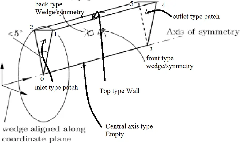
Wedge consists of 6 vertices with 5 faces
- inlet face type patch
- outlet face type patch
- Front face type wedge
- Backface type wedge
- pipe surface face type wall
edge type empty
/*--------------------------------*- C++ -*----------------------------------*\
  =========                 |
  \\      /  F ield         | OpenFOAM: The Open Source CFD Toolbox
   \\    /   O peration     | Website:  https://openfoam.org
    \\  /    A nd           | Version:  8
     \\/     M anipulation  |
\*---------------------------------------------------------------------------*/
FoamFile
{
    version     2.0;
    format      ascii;
    class       dictionary;
    object      blockMeshDict;
}
// * * * * * * * * * * * * * * * * * * * * * * * * * * * * * * * * * * * * * //

 convertToMeters 1;

 vertices
 (
     (     0.000000       0.000000       0.000000)  // point 0
     (     0.000000       0.004998      -0.000131)  // point 1
     (     0.000000       0.004998       0.000131)  // point 2
     (     1.510000       0.000000       0.000000)  // point 3
     (     1.510000       0.004998      -0.000131)  // point 4
     (     1.510000       0.004998       0.000131)  // point 5

 );
 blocks
 (
       hex (0 3 4 1 0 3 5 2)  (200 50 1)  simpleGrading (1.0 0.2 1.0)
 );

 edges
 (
 	 arc 1 2 (0 0.005 0)
 	 arc 4 5 (1.510 0.005 0)
 );

 boundary
 (

 	 inlet
 	{
 	   type patch;
 	   faces
 	   (
 		(0 1 2 0)
	   );
	}

 	 outlet
 	{
 	   type patch;
 	   faces
 	   (
 		(3 5 4 3)
	   );
	}

 	 front
 	{
 	   type wedge;
 	   faces
 	   (
 		(0 3 4 1)
	   );
	}

 	 back
 	{
 	   type wedge;
 	   faces
 	   (
 		(0 2 5 3)
	   );
	}

 	 pipeSurface
 	{
 	   type wall;
 	   faces
 	   (
 		(1 4 5 2)
	   );
	}

 	 centralAxis
 	{
 	   type empty;
 	   faces
 	   (
 		(0 3 3 0)
	   );
	}
);

 mergePatchPairs
(
 );

// * * * * * * * * * * * * * * * * * * * * * * * * * * * * * * * * * * * * * //
Case setup & simulation procedure in OpenFOAM:
- copy icoFoam Tutorial to Run Folder using Terminal.
- Go to the system folder and paste blockMeshDict file into the system folder remove unnecessary extensions.
- Edit contronDict file according to velocity and pipe length time 't' `t > L/U_max` dt should be small enough.
- Edit transportProperties in constant folder.
- Edit initial conditions for pressure and velocity in '0' folder
- velocity equals to average velocity
- type icoFoam to run the setup.
ControlDict file:
/--------------------------------- C++ -----------------------------------\
  =========                 |
  \\      /  F ield         | OpenFOAM: The Open Source CFD Toolbox
   \\    /   O peration     | Website:  https://openfoam.org
    \\  /    A nd           | Version:  8
     \\/     M anipulation  |
\---------------------------------------------------------------------------/
FoamFile
{
    version     2.0;
    format      ascii;
    class       dictionary;
    location    "system";
    object      controlDict;
}
// * * * * * * * * * * * * * * * * * * * * * * * * * * * * * * * * * * * * * //

application     icoFoam;

startFrom       startTime;

startTime       0;

stopAt          endTime;

endTime         0.5;

deltaT          0.05;

writeControl    timeStep;

writeInterval   100;

purgeWrite      0;

writeFormat     ascii;

writePrecision  6;

writeCompression off;

timeFormat      general;

timePrecision   6;

runTimeModifiable true;


// ************************* //
TransportProperties file:
/--------------------------------- C++ -----------------------------------\
  =========                 |
  \\      /  F ield         | OpenFOAM: The Open Source CFD Toolbox
   \\    /   O peration     | Website:  https://openfoam.org
    \\  /    A nd           | Version:  8
     \\/     M anipulation  |
\---------------------------------------------------------------------------/
FoamFile
{
    version     2.0;
    format      ascii;
    class       dictionary;
    location    "constant";
    object      transportProperties;
}
// * * * * * * * * * * * * * * * * * * * * * * * * * * * * * * * * * * * * * //

nu              [0 2 -1 0 0 0 0] 0.00089;


// ************************* //
Velocity file:
/--------------------------------- C++ -----------------------------------\
  =========                 |
  \\      /  F ield         | OpenFOAM: The Open Source CFD Toolbox
   \\    /   O peration     | Website:  https://openfoam.org
    \\  /    A nd           | Version:  8
     \\/     M anipulation  |
\---------------------------------------------------------------------------/
FoamFile
{
    version     2.0;
    format      ascii;
    class       volVectorField;
    object      U;
}
// * * * * * * * * * * * * * * * * * * * * * * * * * * * * * * * * * * * * * //

dimensions      [0 1 -1 0 0 0 0];

internalField   uniform (0.1875 0 0);

boundaryField
{
     inlet
    {
        type            fixedValue;
        value           uniform (0.1875 0 0);
    }

    outlet
    {
        type            zeroGradient;
    }

    front
    {
        type            wedge;
    }

    back
    {
        type            wedge;
    }

    pipeSurface
    {
        type            noSlip;
    }

    centralAxis
    {
        type            empty;
    }
}

// ************************* //
Pressure file:
/--------------------------------- C++ -----------------------------------\
  =========                 |
  \\      /  F ield         | OpenFOAM: The Open Source CFD Toolbox
   \\    /   O peration     | Website:  https://openfoam.org
    \\  /    A nd           | Version:  8
     \\/     M anipulation  |
\---------------------------------------------------------------------------/
FoamFile
{
    version     2.0;
    format      ascii;
    class       volScalarField;
    object      p;
}
// * * * * * * * * * * * * * * * * * * * * * * * * * * * * * * * * * * * * * //
dimensions      [0 2 -2 0 0 0 0];

internalField   uniform 0;

boundaryField
{
    inlet
    {
        type            zeroGradient;
    }

    outlet
    {
        type            fixedValue;
        value           uniform 0.1012;
    }

    front
    {
        type            wedge;
    }

    back
    {
        type            wedge;
    }

    pipeSurface
    {
        type            zeroGradient;
    }

    centralAxis
    {
        type            empty;
    }
}

// ************************* //
Mesh:
Basic statistics
Number of internal faces : 0
Number of boundary faces : 6
Number of defined boundary faces : 6
Number of undefined boundary faces : 0
Checking patch -> block consistency
Creating block offsets
Creating merge list .
Creating polyMesh from blockMesh
Creating patches
Creating cells
Creating points with scale 1
Block 0 cell size :
i : 0.00755 .. 0.00755
j : 0.000200334 .. 4.00668e-05
k : 0 0 3.4938e-05 3.4938e-05
Writing polyMesh
----------------
Mesh Information
----------------
boundingBox: (0 0 -0.000436) (1.51 0.004981 0.000436)
nPoints: 20301
nCells: 10000
nFaces: 40050
nInternalFaces: 19750
----------------
Patches
----------------
patch 0 (start: 19750 size: 50) name: inlet
patch 1 (start: 19800 size: 50) name: outlet
patch 2 (start: 19850 size: 10000) name: front
patch 3 (start: 29850 size: 10000) name: back
patch 4 (start: 39850 size: 200) name: pipeSurface
patch 5 (start: 40050 size: 0) name: centralAxis

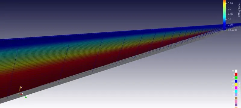
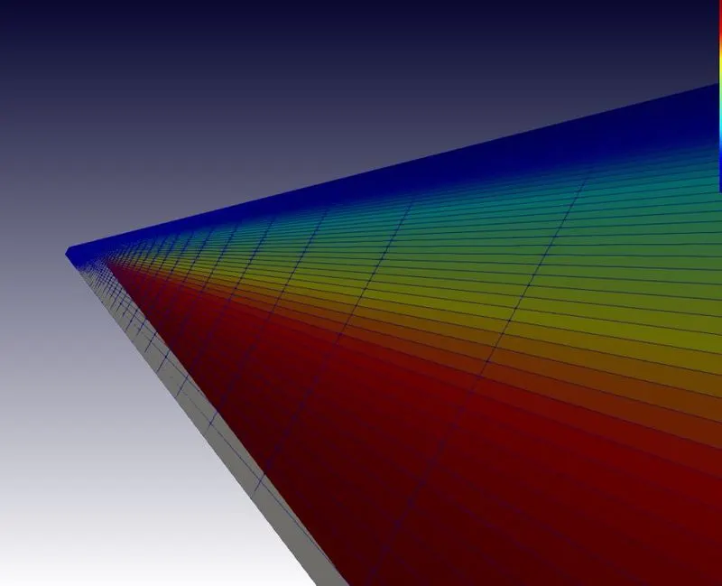
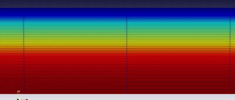
Post Processing of results in ParaView:
- Create slice along with Z normal.
- Use plot over line Command to Plot Velocity profiles at various cross-sectional locations along the length of pipe.
- use Calculator to calculate Shear stress at Fully developed flow section.
- `tau = mu((dU)/dy)` `mu = text(dynamic viscosity ) ; (dU)/dy= text(Gradient)`
- Gradient can be calculated by using command GradientOfUnstructuredDataSet1 in Paraview.
Numerical Plots:
Analytical plots:
Velocity profile video
https://drive.google.com/file/d/1tSVwRC_9i3F_MwyHPfkQf9VbMDKoPu9d/view?usp=sharing
Result Table:
| Maximum velocity | Pressure drop | Maximum Shear Stress | |
| Analytical Solution | 0.3749 | 0.01338 | 0.1335 |
| Numerical Solution | 0.371503 | 0.013405 | 0.130463 |
| error | 0.003397 | 4.749e-04 | 0.003037 |