Week 11: Project 2 - Emission characterization on a CAT3410 engine
Emission characterization on a CAT3410 engine
Aim:- Simulating CAT3410 engine for two different piston configurations. Evaluating different engine parameters and emissions.
Diesel Direct injection:-
Diesel Direct Injection (DI) is a basic type of fuel injection system which is used in diesel engines. The simple DI diesel engines inject the fuel into the combustion chamber above the piston directly. The compression of air inside the combustion chamber raises its temperature above 400oC. Then, it ignites the diesel fuel injected into the combustion chamber. Hence, diesel engines are also known as compression ignition engines.
Flow simulation in CONVERGE is done in 3 steps:
- Geometry preparation and Case setup :
- We use Converge GUI(Graphical User Interface) to set up the case and export input files.
- Solving the problem using input files:
- These input files are solved by Converge in the Terminal (Command-line interface). We USed Cygwin for the command line terminal.
- Post-processing results:
- We convert our solution into Paraview binary format to post-process the results in Paraview
Procedure:
- Geometry preparation:
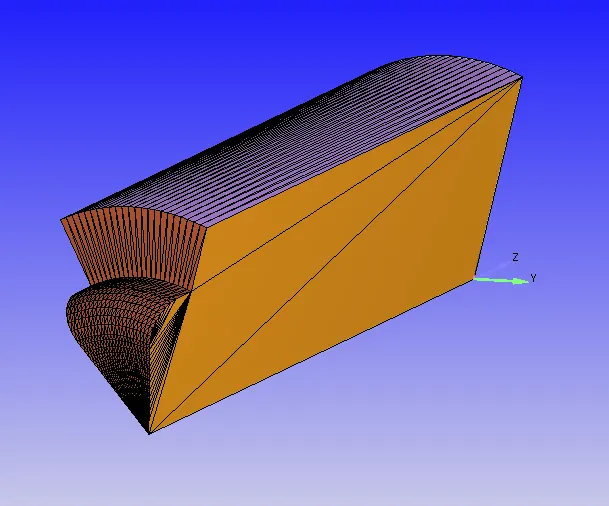
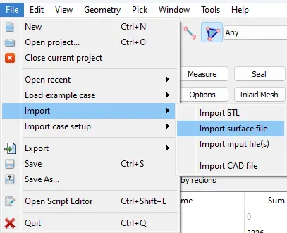
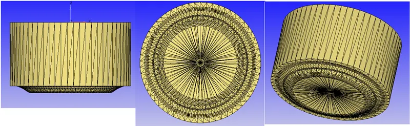
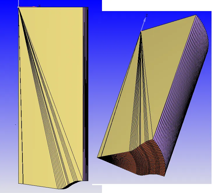
- Import the given surface file "open-w-piston360.dat" which contains the complete piston and cylinder region setup.
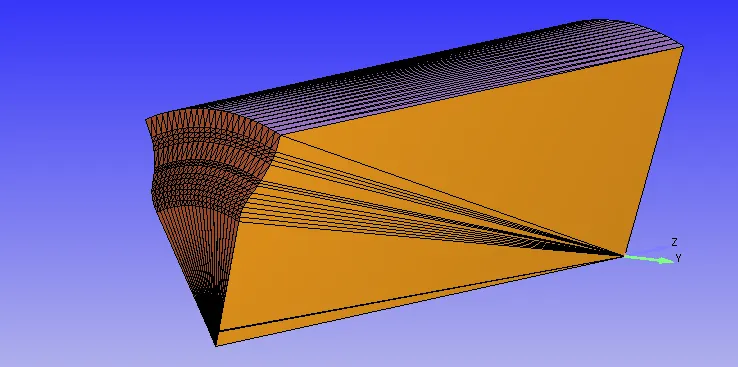
- The above geometry contains only piston head, cylinder liner, and cylinder head surfaces to make it a closed region.
- This is a closed-cycle analysis where we don't need valves or ports for analysis. this increases computation efficiency because we neglected all unnecessary calculations.
- The injector is placed at the center of the cylinder head and contains multiple nozzles.
- In this simulation, we are taking one sector of the domain and simulating combustion in that sector this further decreases the computation power required and the computation time.
- Import the given surface file "open-w-piston360.dat" which contains the complete piston and cylinder region setup.
- Making sector surfaces:
- Tools => Make engine sector surface.
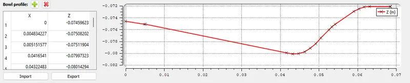
- Extract profile from surface.dat
- Select surface.dat file = open_w_piston_360.dat file
- Extract
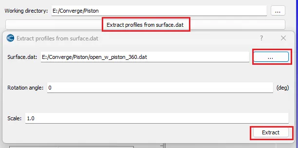
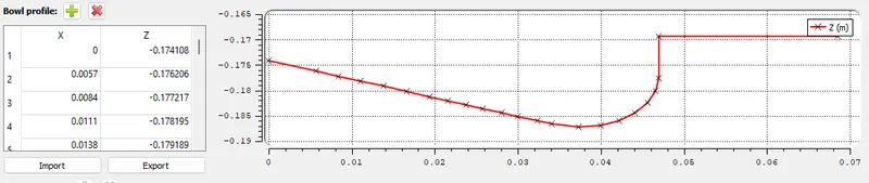
- This creates a bowl profile from the surface file.
- Tools => Make engine sector surface.
- Importing Open-w & Omega piston Bowl profiles:
- Geometric parameters are the same for Omega and Open-w piston bowl profiles.
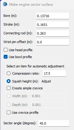
- Open-w-piston:
- Omega Piston:
- For the omega piston, we don't need any surface extraction omega bowl profile is given.
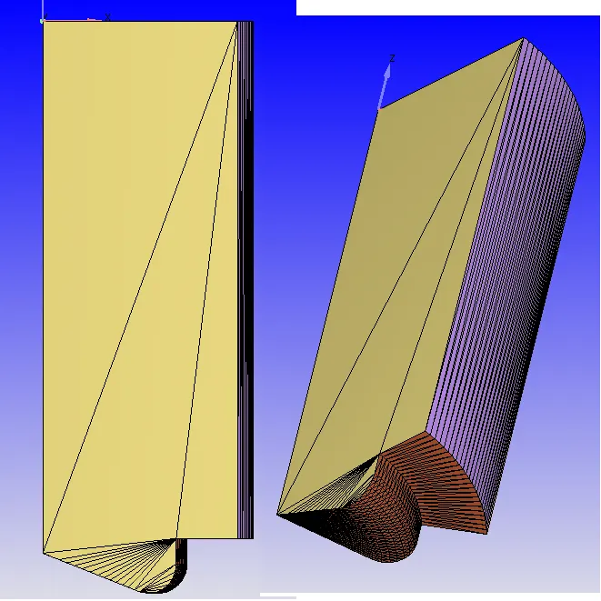
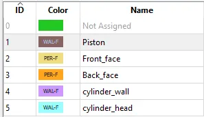
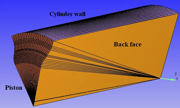
- Boundary Flaging:
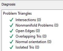
- Run Final Diagnosis: No issues found
---------------------------------------------------------------------------------------------------------------------------------------------
Case Setup:
- Importing input files:
- setting up the case by importing the input files that are provided to us.
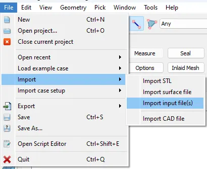
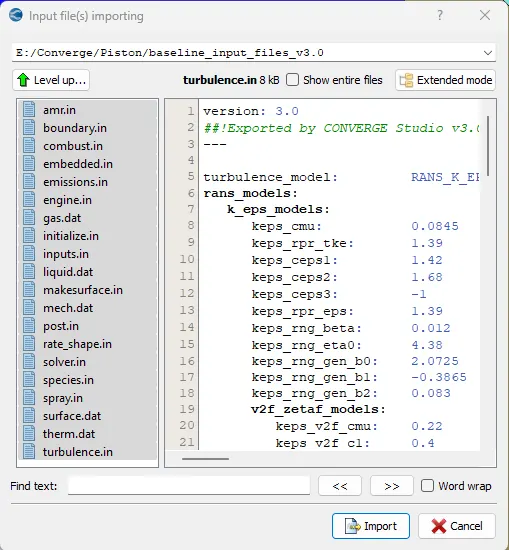
- import all ".in" files
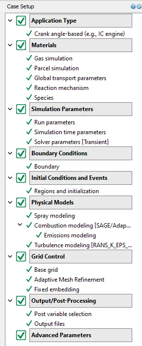
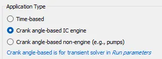
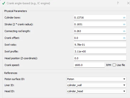
- Application type:
- Materials:
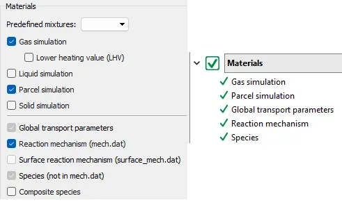
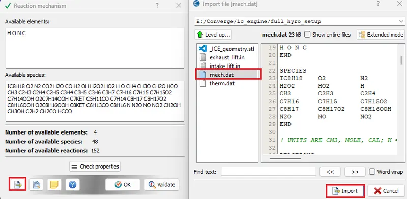
- "mech.dat" file contains gas-phase chemical reactions.
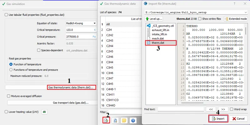
- "therm.dat" file contains the thermodynamic properties of each gas phase.
- Gas Simulation
- Importing Gas Thermodynamic data
- Global transport properties ==>> Default
- Reaction Mechanism:-
- We need to select a reaction mechanism that is compatible with gasoline. JIA PRF(Primary reference fuel) best compactable mechanism for gasoline engines.
- Reaction mechanism => import "mech.dat" file.
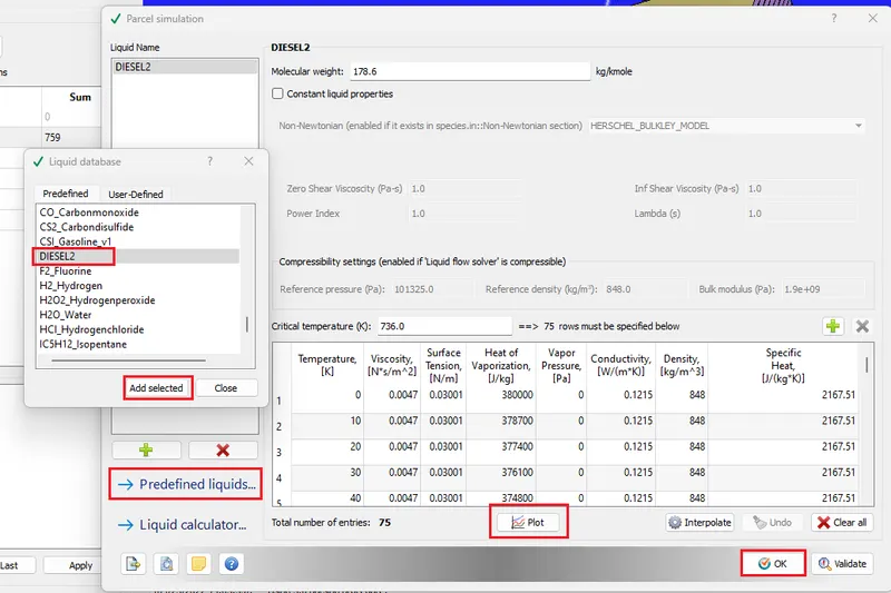
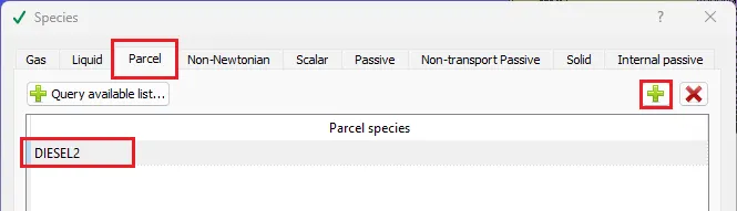
- Parcel Simulation :
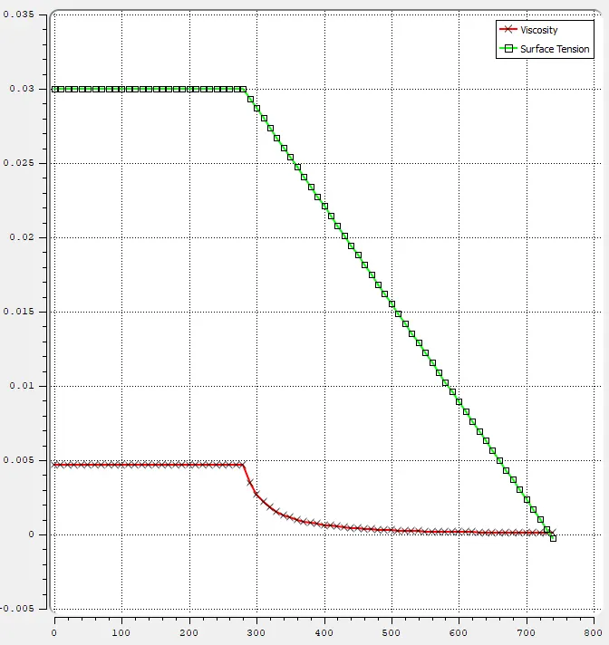
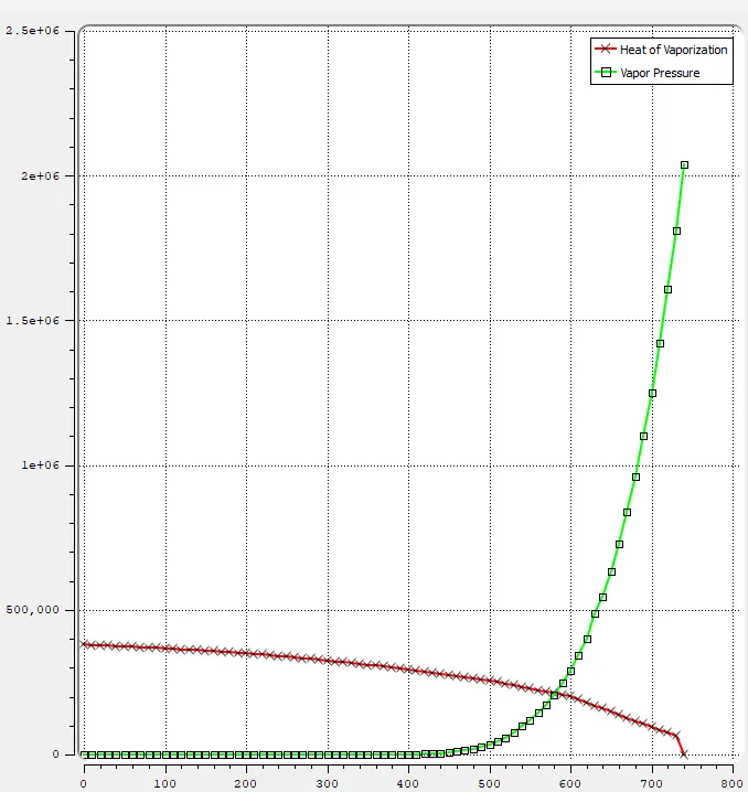
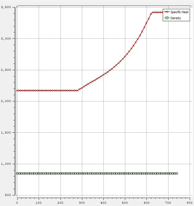
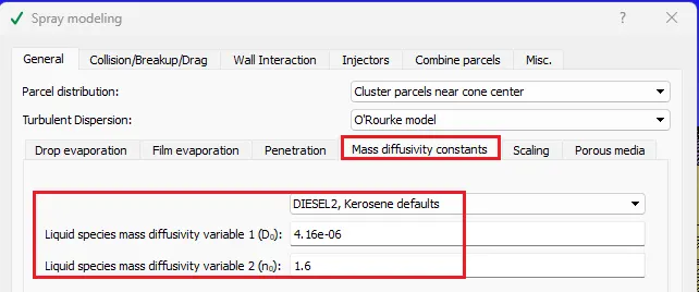
- We have to select the right species for our parcel is made up of. if we don't find the exact fuel species that we are looking for we can use the species whose physical properties match our actual fuel physical properties.
- DIESEL2 has physical properties which are very much closer to Diesel fuel.
- Species:
- We have to add DIESEL2 in the parcel section.
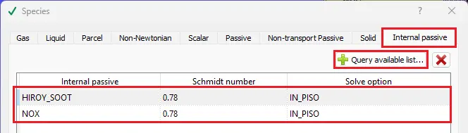
- Adding Hiroy soot and NOx in internal passive.
- Internal Passive in the species consists of all the emission-related gases to be tracked.
- We have to add DIESEL2 in the parcel section.
- Gas Simulation
- Simulation Parameters:
- Run Parameters:
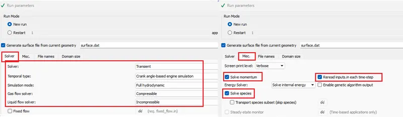
- Transient, Crank angle-based engine simulation with Full Hydrodynamic solution mode.
- In the Full Hydrodynamic case, all the equations are going to be solved.
- Gas is compressible and liquid is incompressible.
- Solve momentum, & Species.
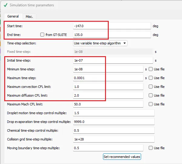
- Simulation Time Parameters:
- Start at -147 degrees till +135 = 282 degrees
- Even though it is not a complete four-stroke cycle, we need only the combustion and emission part of it since no valves are involved in this simulation.
 \
\
- Solver Parameters:
- Run Parameters:
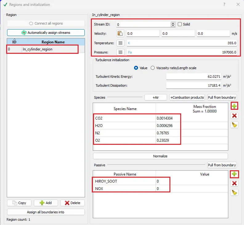
- Initial Conditions and events:

- Defining the regions and solution initialization conditions.
- Boundary Conditions:
-

- Assigning regions to boundary surfaces.
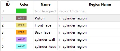
- Boundary condition defines the role of surface in the simulation and assigns what type & certain values to it.
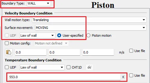
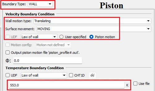
- Piston:
- The Piston is under Translating motion, we have pre-defined piston motion that can be enabled for piston motion for this Piston wall boundary.
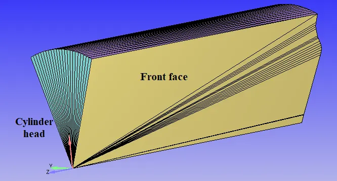
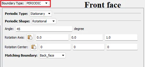
- Front face:
-
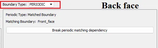
- Back face:
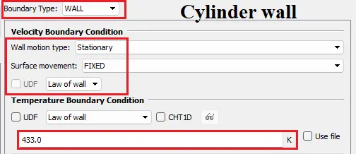
- Cylinder wall:
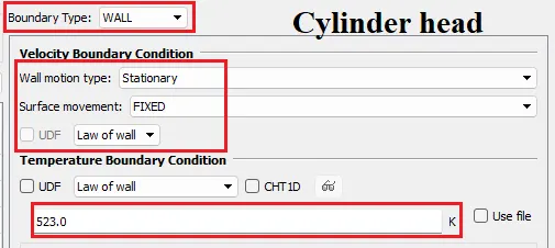
- Cylinder head:
-
- Physical Models:
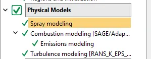
- In Physical models, we have to enable Spray modeling, Combustion modeling, Emission, & Turbulence modeling.
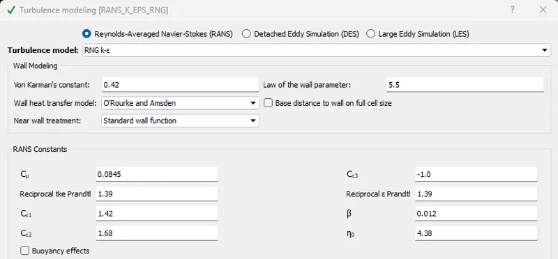
- Turbulence modeling :
- RNG K-`epsilon`
- Spray Modeling:
- Spray modeling:- it is required to specify how the spray of the fuel will propagate in the cylinder and what type of fuel is going to be sprayed. We use models for the simulation of the fuel to get near accurate results and computation time consumption will be less than direct numerical simulation. We spray fuel as lagrangian parcels.
- General:
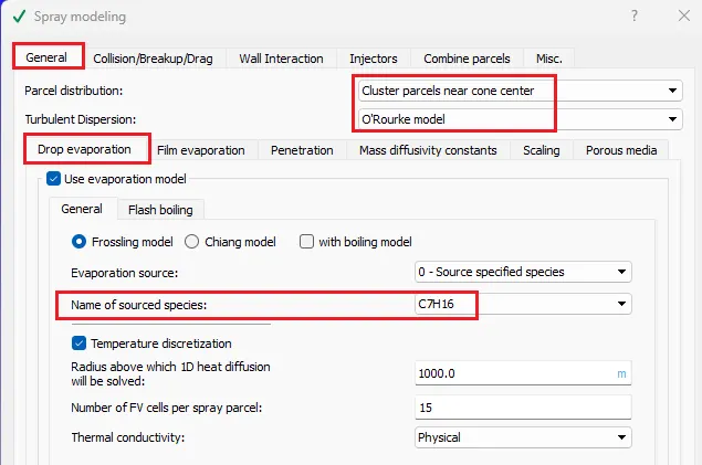
- Diesel parcels are clustered near the cone center.
- We have turbulence in the gas phase this turbulence fluctuations can affect the droplet characteristics. O'Rourke model is preferred.
- C7H16 is used as diesel spray.
- Basically, our fuel parcels are in a spherical shape, the outside of the sphere is much hotter than the inside of the sphere. We can basically discretize the droplet into a number of spherical finite volume cells and solve heat ODE equations in all of those individual finite volume cells. In our case, we are not interested in solving this because we don't need that level of accuracy that's why we are considering our droplets are of one temperature. It can be achieved by using a larger value for the radius so that ode is never solved. ODE is solved when the parcel radius is more than the specified radius.
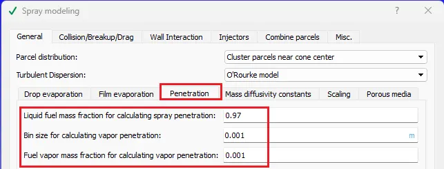
- Liquid fuel mass fraction for calculating spray penetration = 0.97
- liquid penetration length is calculated till fuel mass is equal to 97% of the actual fuel injected.
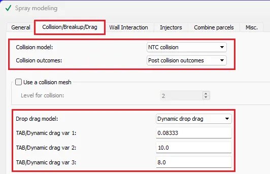
- Collision/Breakup:
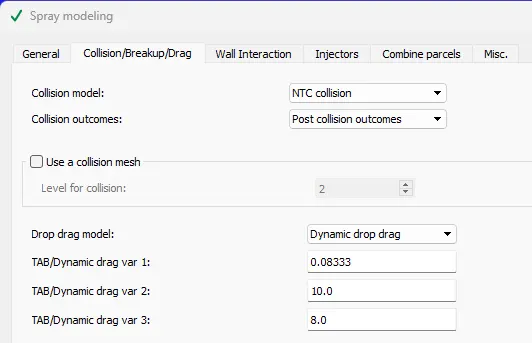
- Once the fuel is injected at very high pressure, fuel parcels are scattered and they go through different phases like collision, break and drag. How things will go on with the parcels can be predicted with the models of collision, drag, and break up models.
- NTC Collision model, Post Collision outcomes.
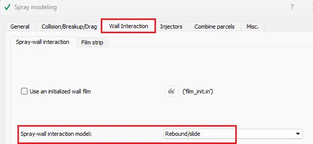
- Wall Interaction:
- Use collision mesh to avoid grid effects.
- Once the fuel is sprayed they travel towards the walls around them and interact. this interaction will lead to different phenomena. However, to make things simple we can specify the way of interaction.
- Injectors:
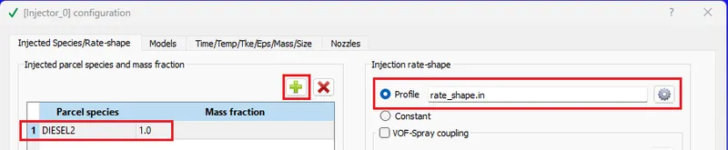
- In order to spray the fuel, we need injectors to be placed inside the cylinder.
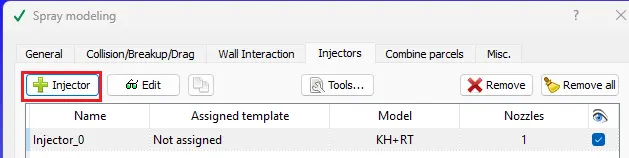
- Adding injector.
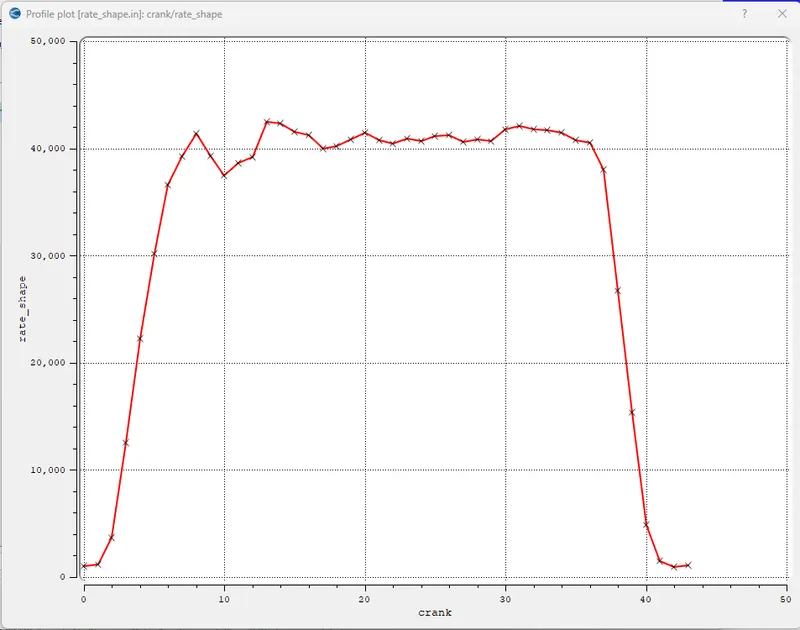
- Injector Species Rate shape = constant.
- Injector parcel Species = Diesel2, Rate shape = profile.
- Models:
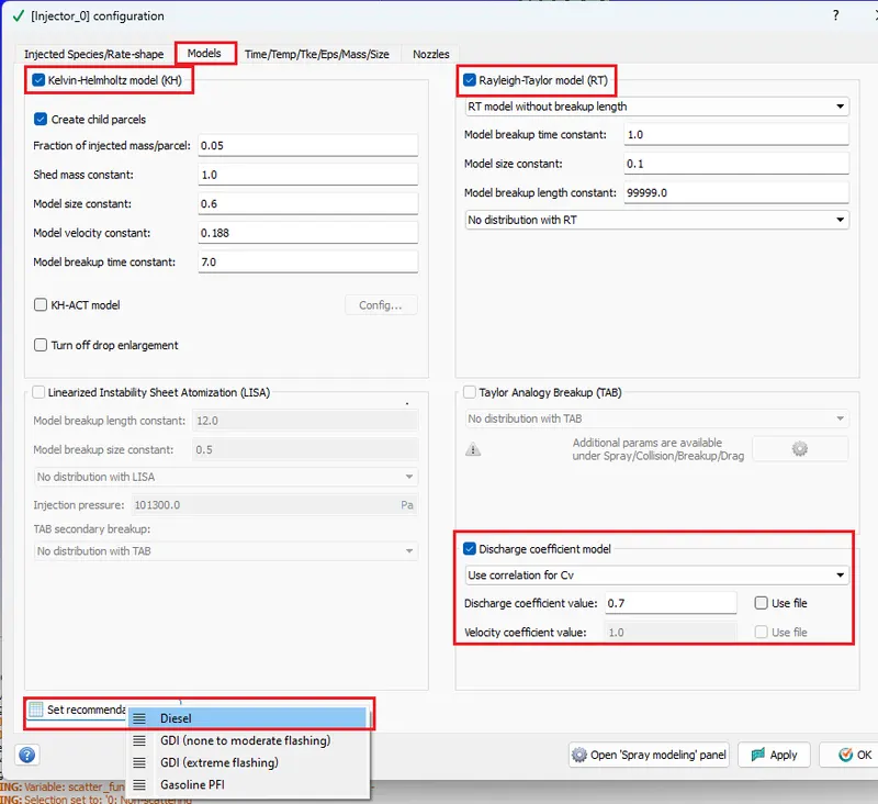
- Kelvin-Helmholtz & Rayleigh-Taylor are the Popular models used for solid cone sprays this model will tell how the injection is to be performed.
- Set recommended values for gasoline fuel.
- These Constant values control how your parcel going to break up.
- Set recommendation settings for Diesel.
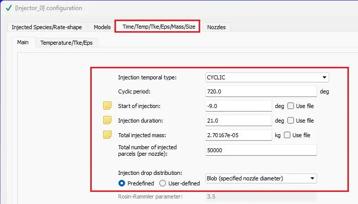
- Temp/time/mass/size
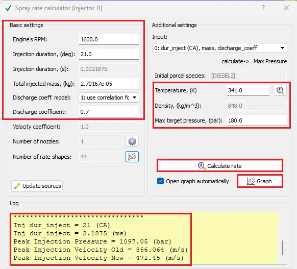
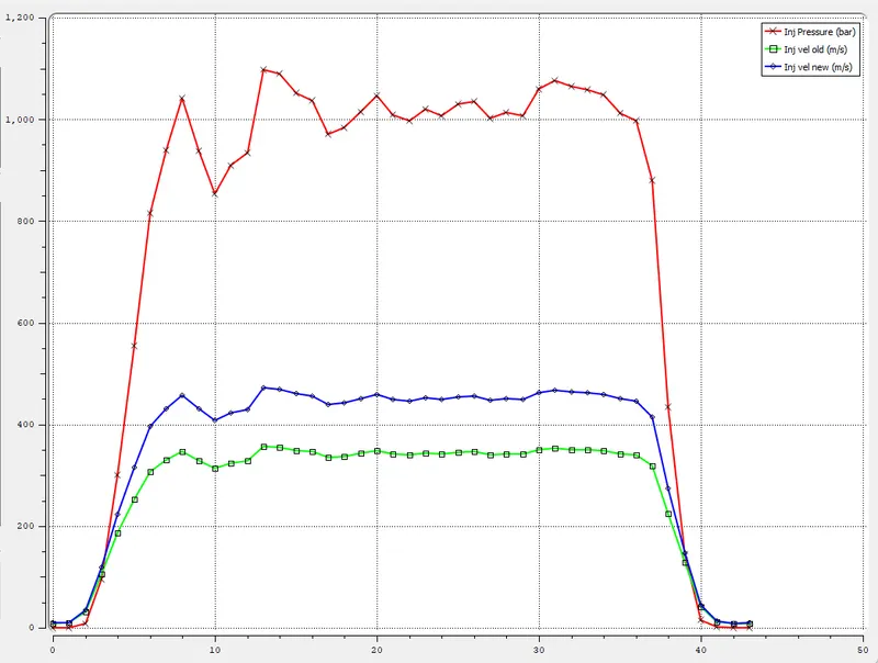
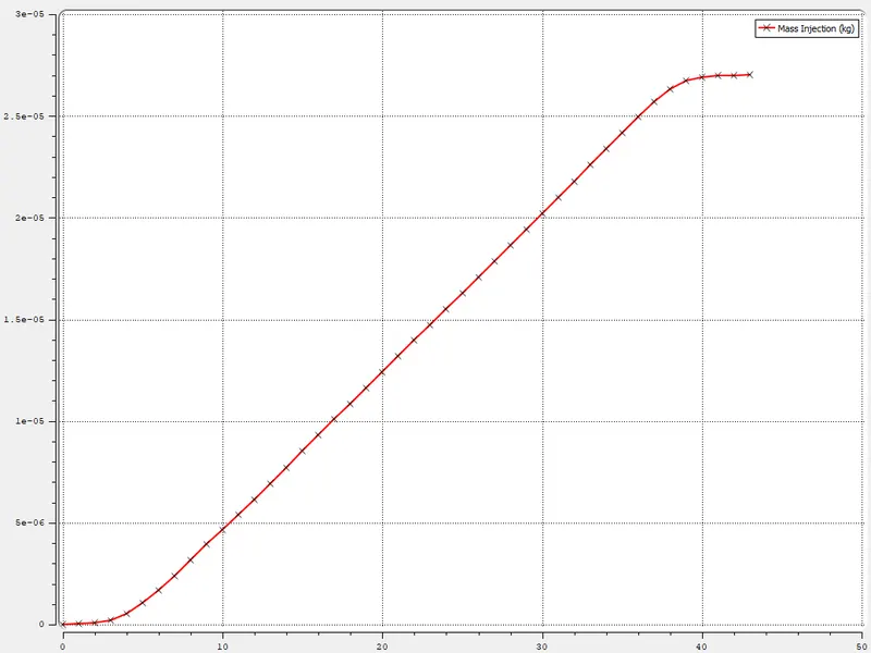
- In the case of the engine, fuel spray does not take place every second it takes place at every cycle. This flow rate can be converted into absolute mass
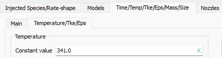
- Nozzles:
- We have 8 nozzles attached to the one injector. in this simulation we are simulating 1/8 sector containing one nozzle in it.
- Nozzle geometry & Location:
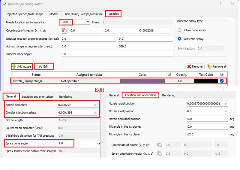
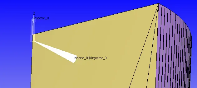
- Validate Nozzle location all nozzles should be inside the computational domain.
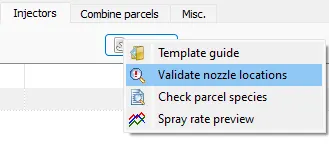
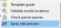
- Spray Rate Preview:
- Combustion modeling:
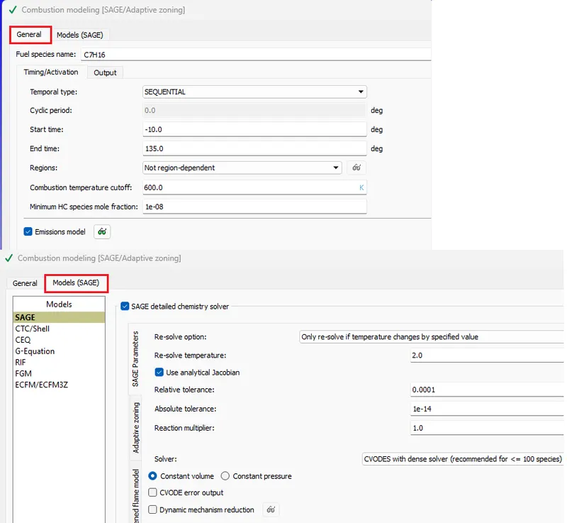
- SAGE combustion Model is used to speed up the combustion calculations.
- Emissions modeling:
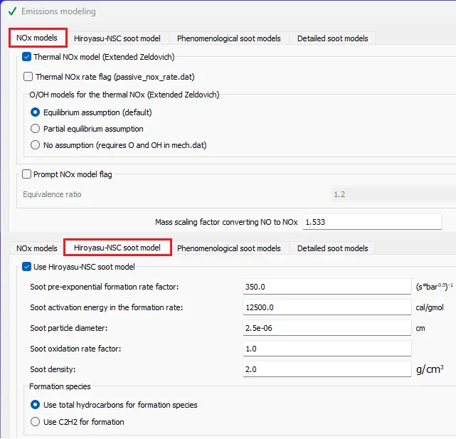
- Emissions play an important role in the performance of the engine. To get accurate results we are going to use approximation models for Hiroy soot and for NOx.
- Turbulence modeling :
- Grid Control:
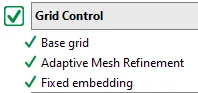
- The meshing part can be done through Grid control.
- Base grid:
- Setting base grid size to 0.004 m or 4 mm

- Fixed Embedding:
- We don't need highly refined mesh in the entire domain this will leads to more computation time to solve every cell, on the same way we cannot use coarse mesh which will take us to inaccurate and wrong results. To overcome this problem we are going to refine the mesh in particular zones or areas where we need more accurate results and physical properties changes rapidly.
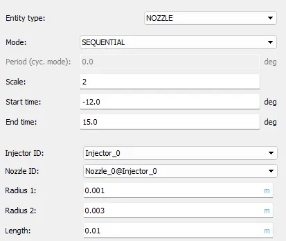
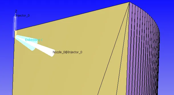
- Embedding around fuel spray:
- When the fuel is injected fuel gets atomized and some portion of the fuel is converted into vapor form for accurate calculation of fuel liquid penetration and vapor penetration we need more refinement around the spray.
- `text(Cell size) = text(Base mesh size)/2^(text(Scale)) = 0.004/2^(2)=0.0001 text( meters)`
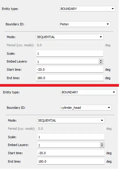
- Sequential Boundary-based Embedding over Piston surface and Cylinder head surface.
- This kind of boundary meshing is created in between a particular period of start and end angle
- This embedding is used to capture accurate wall interaction parameters like fuel rebound, temperature, pressure, etc.
- `text(Cell size) = text(Base mesh size)/2^(text(Scale)) = 0.004/2^(1)=0.0002 text( meters)`
- Embedding around fuel spray:
- We don't need highly refined mesh in the entire domain this will leads to more computation time to solve every cell, on the same way we cannot use coarse mesh which will take us to inaccurate and wrong results. To overcome this problem we are going to refine the mesh in particular zones or areas where we need more accurate results and physical properties changes rapidly.
- Adaptive Mesh refinement (AMR):
- In Adaptive Mesh refinement mesh gets auto-refined according to the condition given.
- here we are specifying the maximum number of cells that can be reached after refinement is 200,000 cells.
- firstly we have to shift the Volumetric_region in available regions to active regions.
- For this case, we are using Velocity & Temperature based AMR so that we can monitor the curvature of Velocity and temperature
- Embed type: Sub-grid Scale (SGS)
- we have to enter magnitude for sub-grid criterion. for example, if we enter Sub-grid criterion = 0.001 mesh gets auto refined in the region where the variable difference between `N_(th)` cell and `(N-1)_(th)` cell is greater than SGS criteria.
- Max embedding level is used to calculate the size of the refined cell.
- `text(Grid size)=text(Base grid size)/2^text(Embed level)`
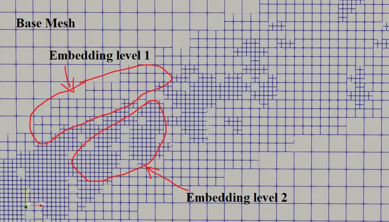
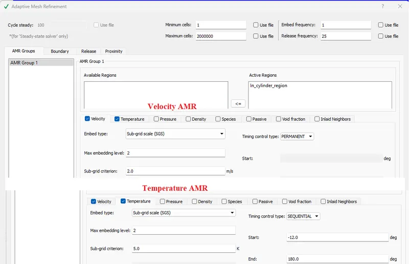
- Velocity AMR is permanent and continuous throughout the simulation.
- Temperature AMR is sequential in nature.
- The meshing part can be done through Grid control.
- Output/Post-Processing
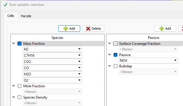
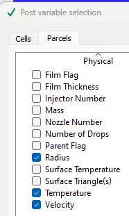
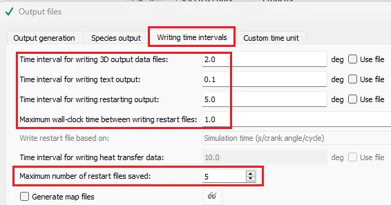
- Post Variable selection: select the variables to be monitored for post-processing.
-
S.No Typical variables Geometry/Location 1 Density Region ID 2 Pressure 3 Temperature 4 Velocity 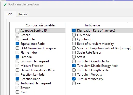
-
- Post Variable selection: select the variables to be monitored for post-processing.
- Exporting Input files:
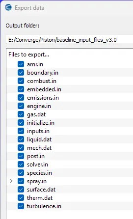
- Export the input files
- Export the input files


---------------------------------------------------------------------------------------------------------------------------------------------
Solving in Cygwin:
- Go to the directory where input files are exported
- Make mpiexec.exe & converge.exe files globally available.
- "mpiexec.exe -n 4 converge.exe restricted </dev/null> logfile &"
- Use above mentioned line to start calculation in the background
- mpiexec.exe & converge.exe are executable applications to solve the problem
- -n 4:- number of processors
- restricted:- my license is a restricted one.
- </dev/null> logfile:- creates temporary memory to save data with name as logfile at a particular iteration
- & :- To run Calculation in Background
- "tail -10 logfile" command is used to view the last 10 lines of the log file.
- "mpiexec.exe -n 1 post_convert_30_serial_64" command used to convert output files to paraview binary format, so that they can be processed in the paraview.
Calculations:
- `text(Power) = text(work)/text(time) text( watt)`
- `text(Torque) =(text(Power)*60)/(2*pi.N) text( N-m)`
- Power developed by the Omega piston engine:
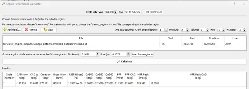
- From engine performance calculator
- work = 3409.28 N.m
- Duration = 270.171 degrees
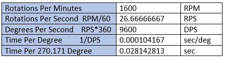
- `text(Power) = text(work)/text(time)= 3409.28/0.028142=121142.1749 text( watt)`
- `text(Torque) =(text(Power)*60)/(2*pi.N) = (121142.1749**60)/(2**pi**1600)= 723.014 text(N-m)`
- Power developed by the Open-w piston engine:
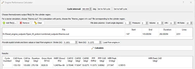
- From engine performance calculator
- work = 3028.53 N.m
- Duration = 270.15 degrees
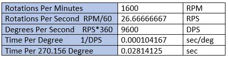
- `text(Power) = text(work)/text(time)= 3028.53/0.028142=107616.0187 text( watt)`
- `text(Torque) =(text(Power)*60)/(2*pi.N) = (107616.0187**60)/(2**pi**1600)= 642.2857 text(N-m)`
- Comparision:
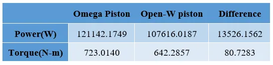
- Here we can see that the Omega piston has generated almost 13.5261 KW more power than the Open-w piston for the same amount of fuel.
Plots :
- Pressure plot:
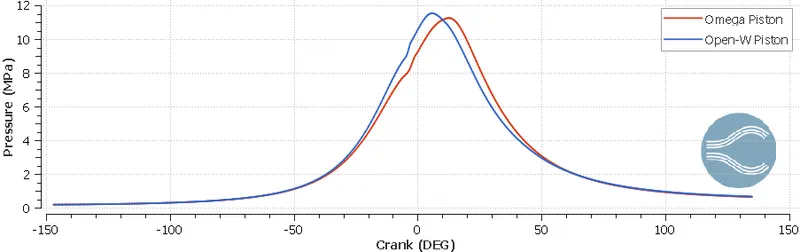
- From the pressure plot, it can be observed during the combustion period the Open-W piston generated little high pressure when compared to the omega piston. At the end, both have similar pressure values.
- The maximum pressure generated when we use the Open-W piston is 11.5372 Mpa whereas Omega piston generated a maximum pressure of 11.2575 Mpa.
- This 0.2729 Mpa difference is due to the bowl profile.
- Mean Temperature:
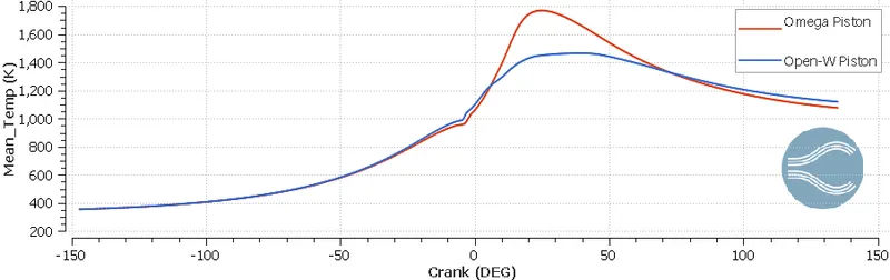
- From the plot, we can observe a sharp increase and decrease in temperature for the omega piston but, for the case of the Open-W piston, we can observe a steady increase and decrease in the temperature. At the end, the Open-W piston maintained a little high temperature than the Omega piston.
- From this, we can conclude that in the case of the omega piston combustion started a bit late but, the fuel is was burnt so quickly.
- The maximum temperature reached by using the Omega piston is 1763.4 K, whereas the maximum temperature reached by the Open-W piston generated 1464.54 K.
- Integrated Heat release:
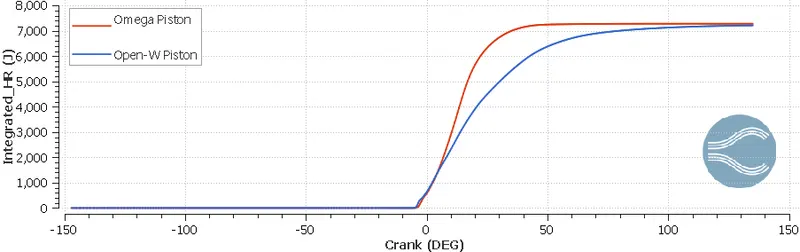
- Integrated heat release means the amount of heat that is generated per cycle.
- Omega Piston has a clear-up hand in the amount of integrated heat released is equal to 7279.46 J whereas for Open-W piston 7211.54 J of heat released.
- The difference in the amount of heat released is about 67.92 J. It looks small difference for a single cycle but when we calculate for more cycles it definitely matters a lot. For 1000 cycles we will get a difference of 67.92 KJ.
- Heat release rate:
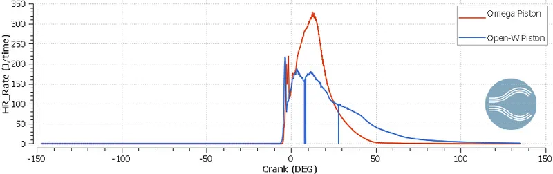
- Heat release rate tells us the amount of heat generated per unit time. omega has a clear and smoother profile than that of open-w. The open-w profile is quite unpredictable and this tells that there are lot of incomplete burning of the gases is taking place.
Emission Plots:
- Hiroy Soot:
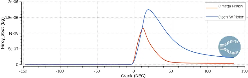
- Soot is a mass of impure carbon particles resulting from the incomplete combustion of hydrocarbons.
- From the soot plot, it is clear that the formation of soot is very high in the case of an Open-W piston.
- Omega = 3.39162e-8 Kg; Open-W = 2.21866e-7 Kg.
- NOx:
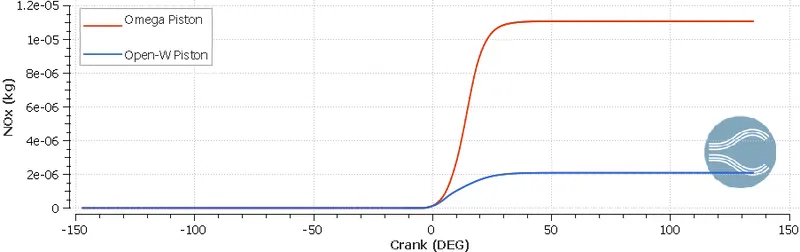
- NO x is a generic term for the nitrogen oxides that are most relevant for air pollution, namely nitric oxide(NO) and nitrogen dioxide(NO 2 ).
- Omega piston produces a high quantity of NOx than Open-W this is because Omega piston developed and operated at high temperature leads to the formation of a high amount of NOx.
- Omega = 1.10645e-5 Kg; Open-W = 2.0884e-6 Kg.
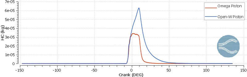
- HC:
- Hydrocarbons(HC) are nothing but Unburnt fuel emitted out of the engine.
- The Amount of Hydro carbons produced for the case of Open-W piston is greater at the beginning of the combustion by the end Hydrocarbon emission was less and closer to each other.
- Omega = 2.1825e-9Kg; Open-W = 6.1011705e-8 Kg.
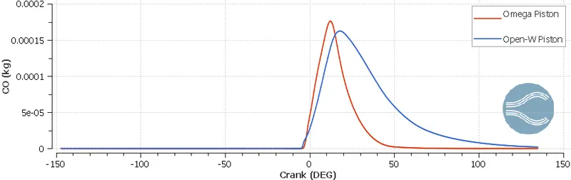
- CO:
- Carbon monoxide is produced during incomplete combustion. Anything that leads to incomplete combustion increases CO production. Two major causes are a rich fuel mixture or restricted air supply.
- Open-W piston emits a little higher quantity of CO than Omega piston.
- Omega = 8.7152e-12 Kg; Open-W = 2.126e-6 Kg.
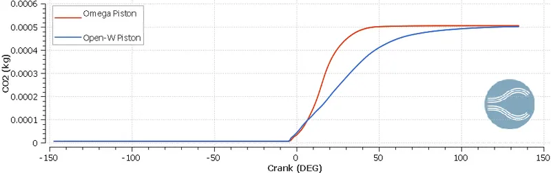
- CO2:
- The burning of fossil fuels produces CO2.
- Both Omega and Open-W piston profiles emit similar amounts of CO2. Out of which Open-W emits somewhat little in quantity.
- Omega = 5.05013e-4 Kg; Open-W = 5.01541e-4 Kg.
CONCLUSION:
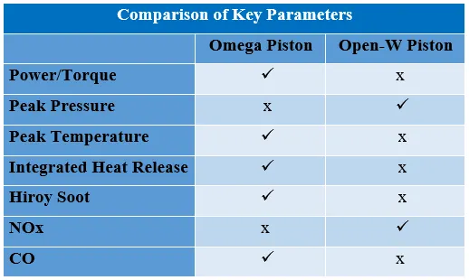
- After comparing all the main output engine parameters Omega piston has more advantages than Open-W piston.
- Omega Piston has clear domination over Open-W piston but omega piston produces more amount of NOx when compared to Open-W.
- Production of Nox and CO2 can be minimized by using after treatments such as exhaust gas recirculation (EGR) and selective catalytic reduction (SCR)
- Percentage of Combustion vs Crank angle:
- CA stands for crank angle, CAD10, CAD50 & CAD90 stand for crank angle in Degrees at 10%, 50% and 90% of combustion happened inside the cylinder.
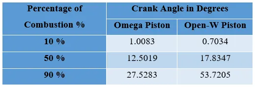
- By observing the above table we can notice that the combustion of fuel started a bit late in the case of the Omega piston but it completed twice fast as the Open-W piston.
- This is the reason for achieving peak temperature and this leads for the formation of more Nox.