Joint creation and Demonstration using LS-DYNA

AIM: To simulate various joints, namely spherical, cylindrical, translational and revolute joints for rigid and deformable bodies using LS-PrePost.

PROCEDURE:

1. Spherical joint:

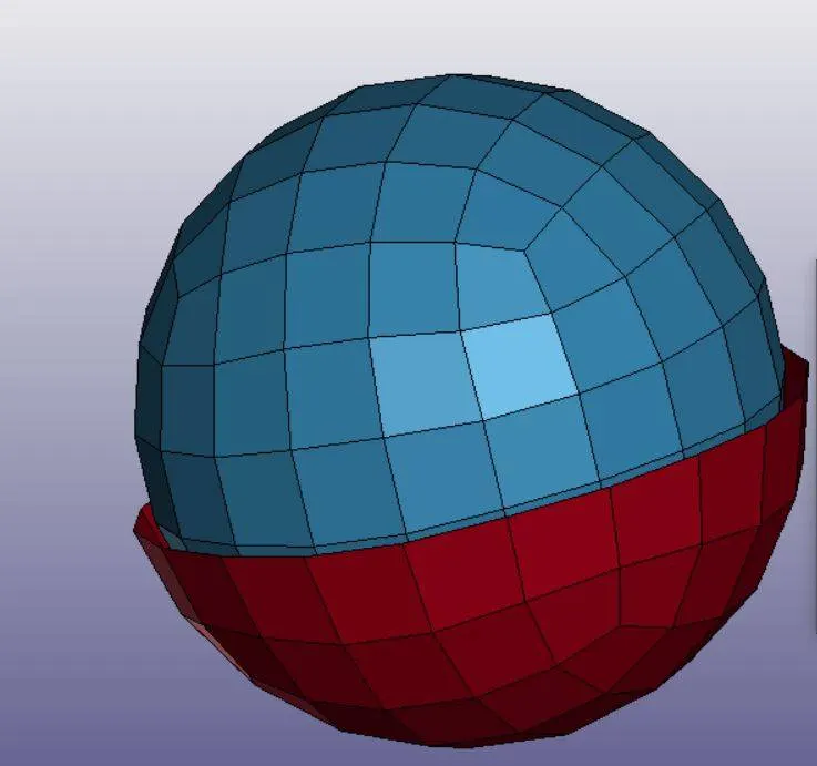
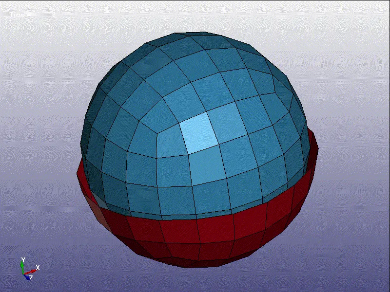
To simulate a spherical joint, initially an outer and inner spherical shell elements were created by going to Elements and Mesh => Shape Mesher => Entity:Sphere Shell. The outer shell was made into hemisphere by deleting one-half of the elements by using Element editing option. The model looks as shown in figure:

Two nodes are created on the centre of the two spheres which are coinciding with each other. This is done by using the Node Editing option.

These nodes need to be assigned to their respective parts. One node is assigned to the outer hemisphere and one node is assigned to the inner sphere.

This can be done for rigid bodies by going to Model and Part => Keyword manager => Constrained => Extra_Nodes_Set.

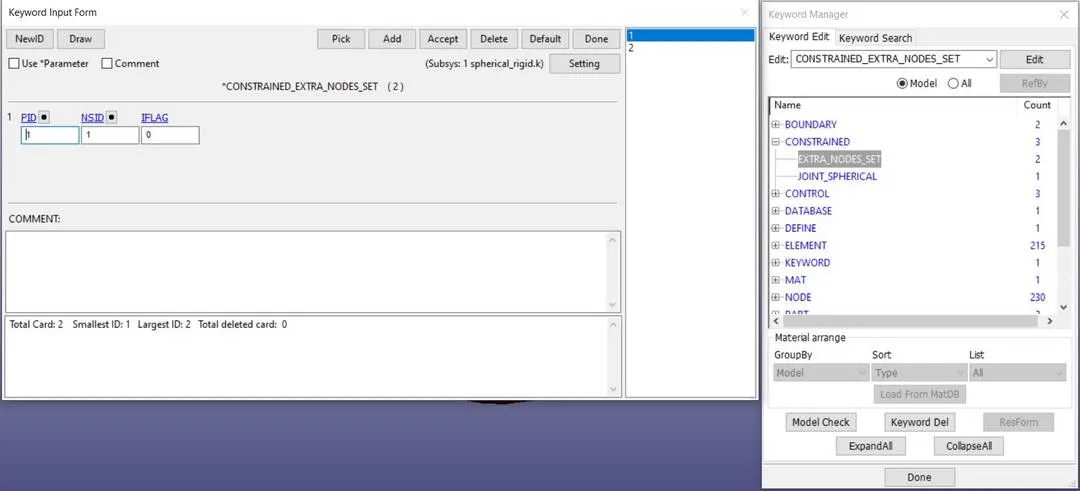
Using this, the respective node is added to the respective part.

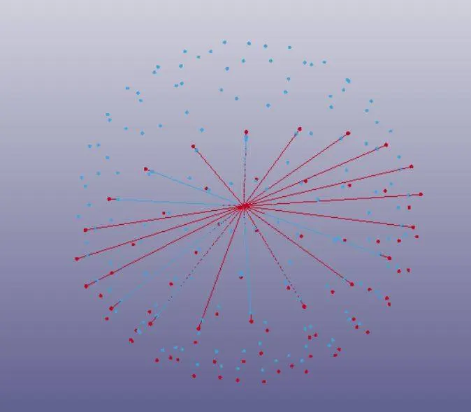
For deformable bodies, this is done by using constrained nodal rigid bodies between the part and the respective node. This can be created by going to Model and Part => Create Entity => Constrained => Nodel Rigid Body (CNRB). This is shown below:

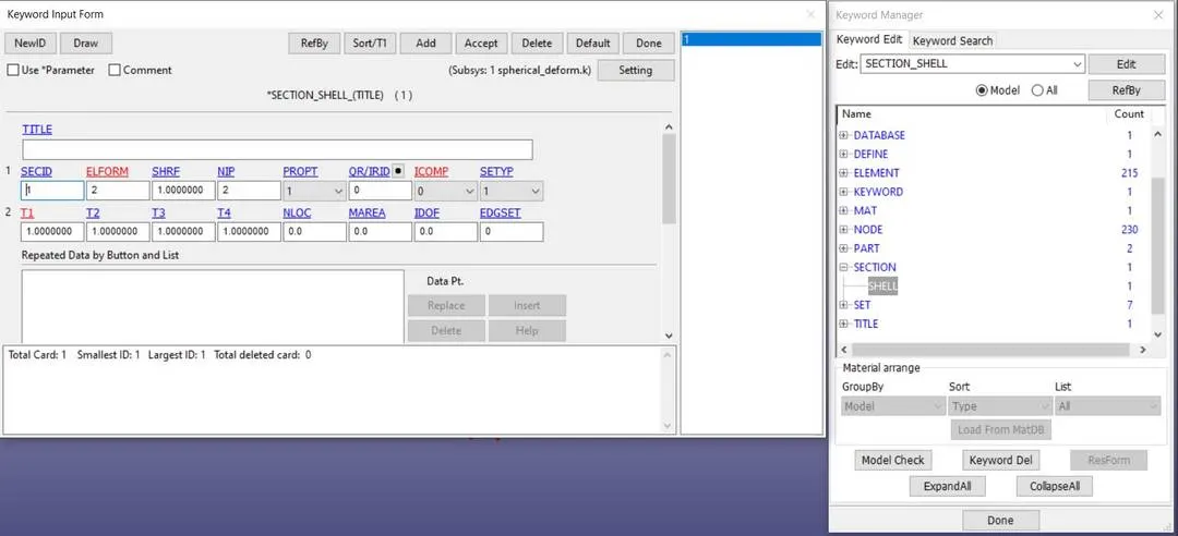
The section properties are given in keyword manager by going to SECTION => SHELL. The properties for both rigid and deformable cases are the same and shown below:

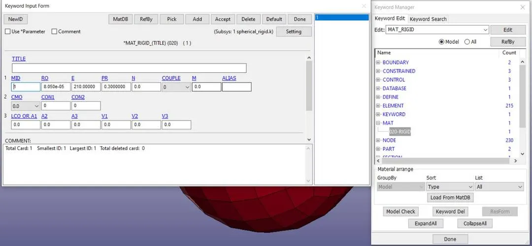
Material properties for rigid body is given by going to MAT => 020-Rigid as shown below:

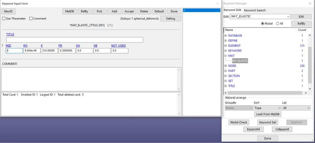
Material properties for deformable bodies is given by going to MAT => 001-Elastic as shown below:

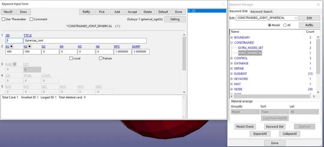
The two nodes at the center are assigned to a spherical joint by going to Constrained => Joint_Spherical as shown below:

Displacement curve is defined by going to DEFINE=> Curve in keyword manager. The displacement curve is shown below:

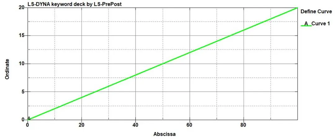
This displacement is given as prescribed motion on one node at the top of the inner sphere. This is then used as a simulation of a simple spherical joint by using implicit analysis mode.

For the case of deformable bodies, the hemisphere's end nodes are constrained by going to Boundary => SPC_Set and all degrees of freedom are constrained.

The result of the rigid joint is shown below:

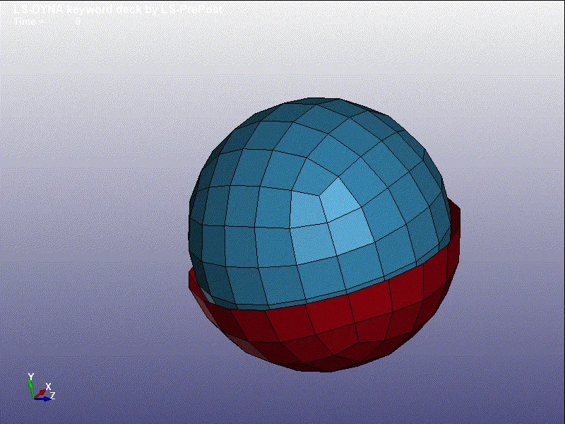
The result of the deformable joint is shown below:

2. Revolute joint:

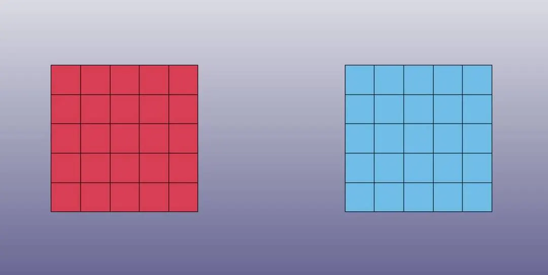
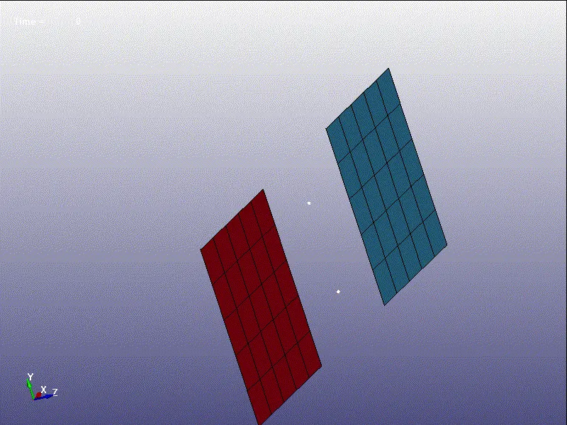
To simulate a revolute joint, two plane shells are created by going to Element and Mesh => Shape Mesher => Entity: 4N Shell. The shells are as shown below:

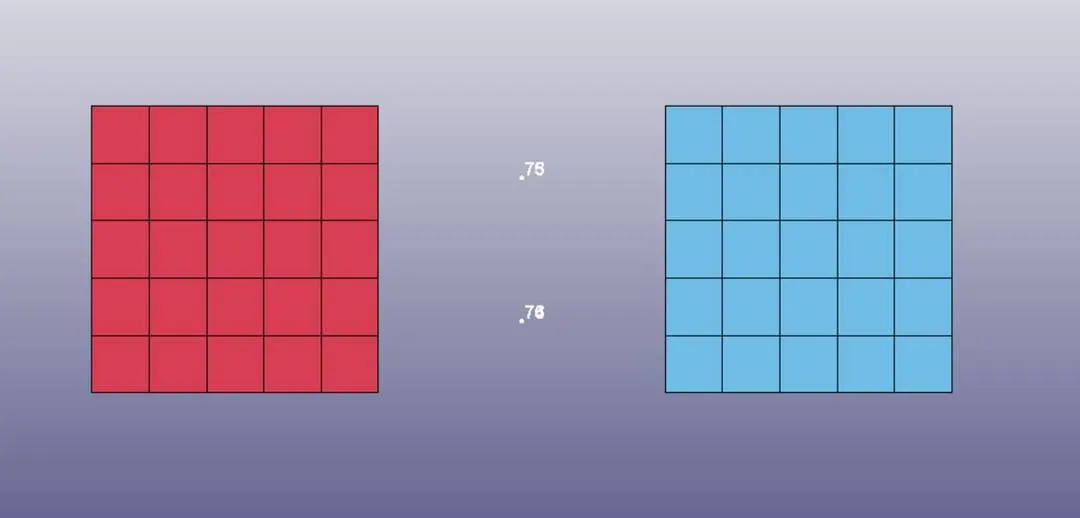
Two nodes for two positions each are created in between the two entities which also fall in the same line as shown below:

One node in each position is assigned to one part respectively as was shown for the spherical joint. For deformable joint, constrained nodal rigid bodies are made as was done in case of spherical joints as shown below:

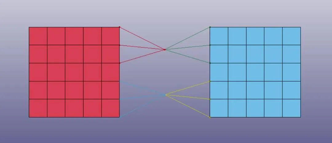
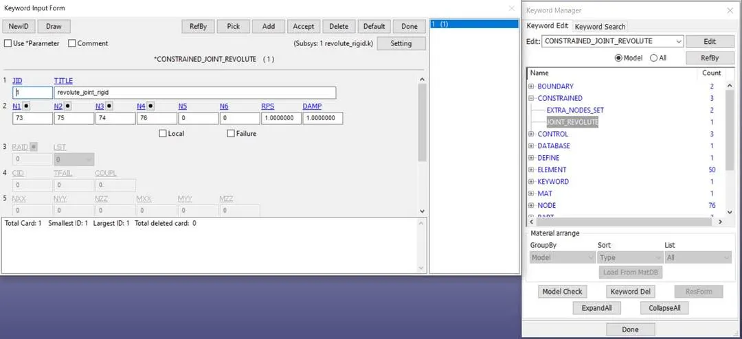
These nodes are also used to create a revolute joint by going to Constrained => Joint_Revolute as shown below:

Material and section properties are given as was done in spherical joints. The boundary conditions are shown below:

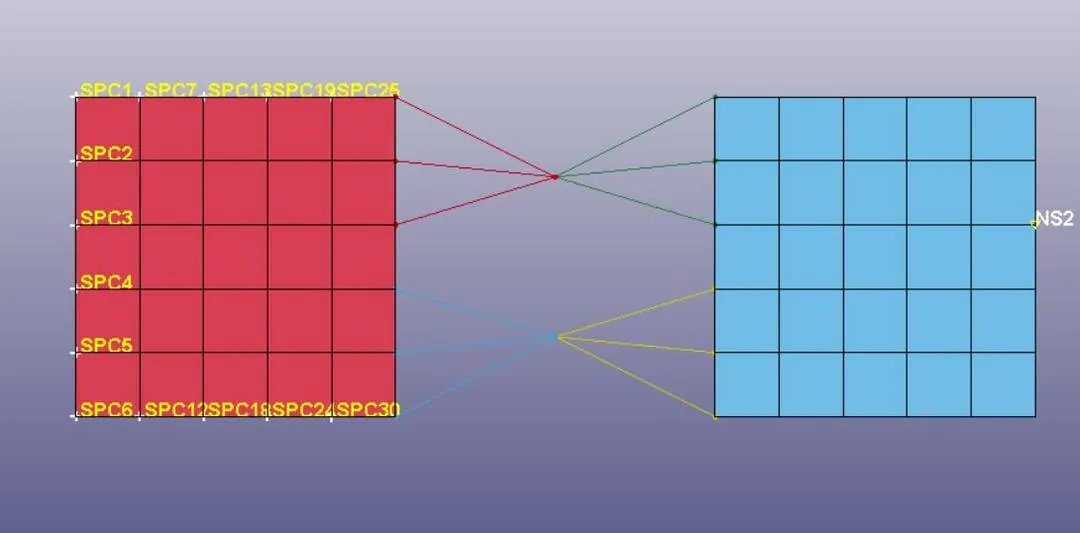
The yellow nodes are constrained in all degrees of freedom. The white node is given prescribed motion. The simulation is done using implicit analysis.

The results from rigid joint is shown below:

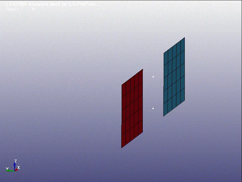
The results from the deformable joint is shown below:

3. Cylindrical joint:

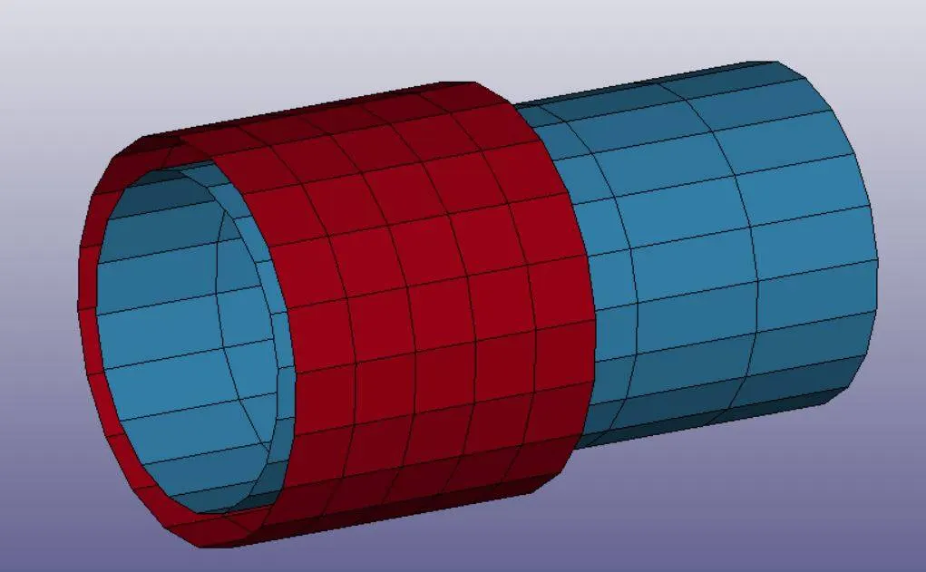
Cylindrical shells are created with one having a larger diameter and the other with a smaller diameter as shown below:

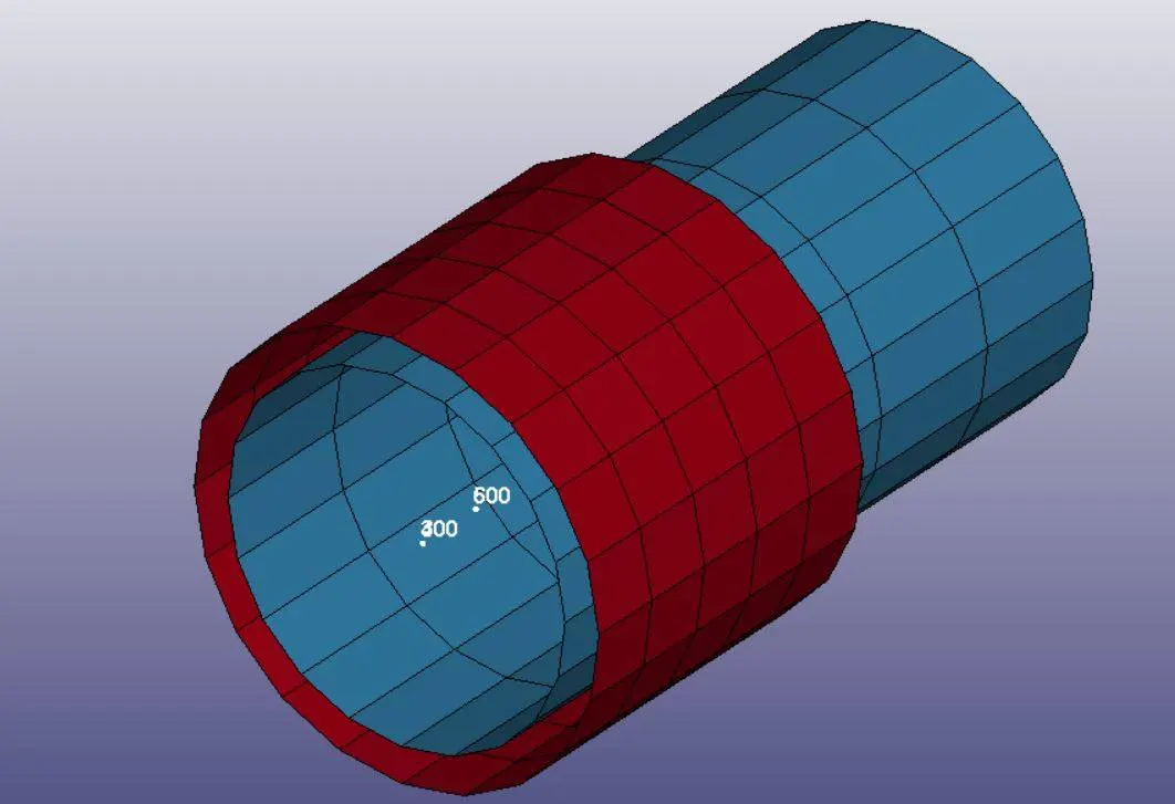
Four nodes are created at the central axis in the same line, similar to the revolute joint as shown below:

In case of rigid bodies, the nodes are assigned to respective parts by going to Constrained_extra_nodes_set and for deformable bodies, constrained nodal rigid bodies are used to connect the nodes to their parts as shown below:

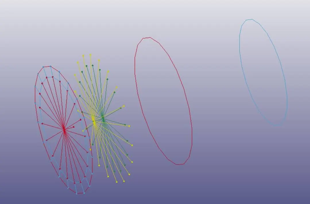
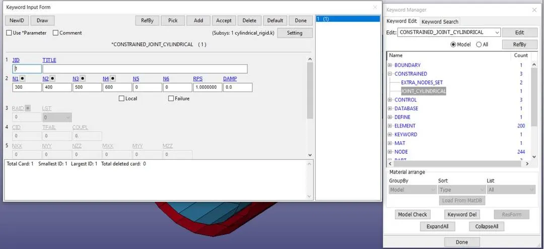
The nodes are assigned to cylindrical joint by going to Constrained => Joint_Cylindrical as shown below:

Boundary conditions for the deformable case are shown below:

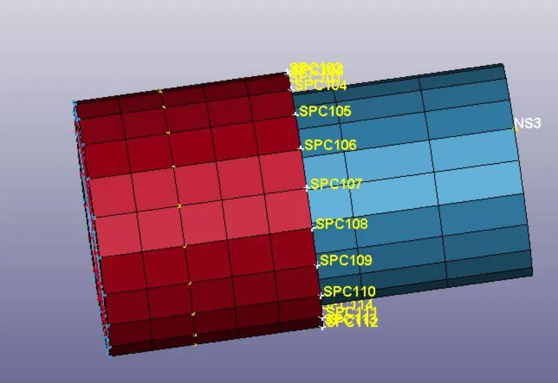
The yellow nodes are constrained for all degrees of freedom and the white node is given translational motion. Implicit analysis is conducted to simulate the joint.

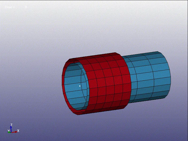
The result of the rigid joint is below:

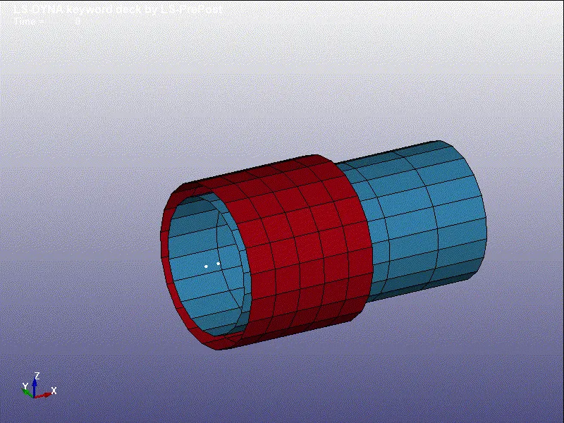
The result of the deformable joint is below;

4. Translational joint:

The models for the translational joint are created by making box shells and deleting opposite faces of one end in order to create a square hole. The model is shown below:

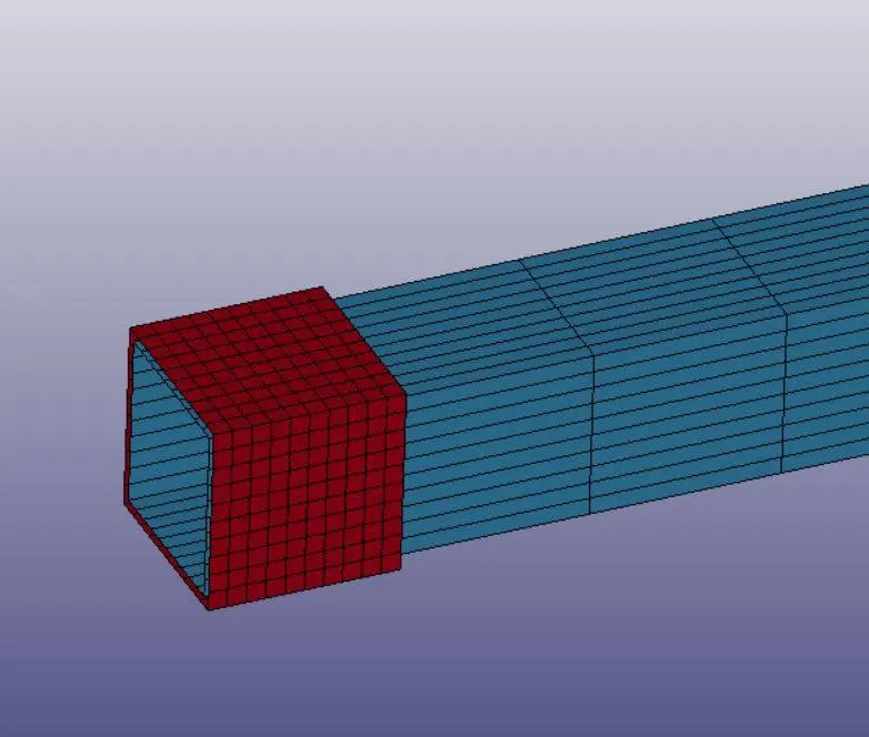
Six nodes are created in the hole with four nodes in the same line as in the case of cylindrical joints whereas the other two nodes are in between these nodes but offset in one dimension as shown below:

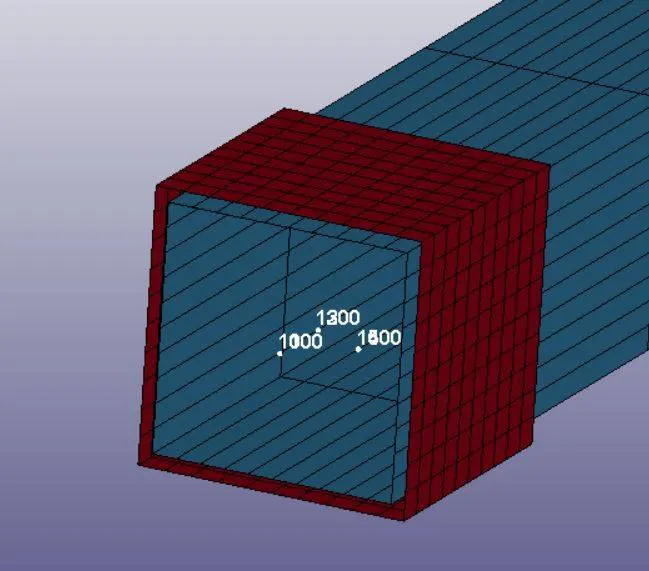
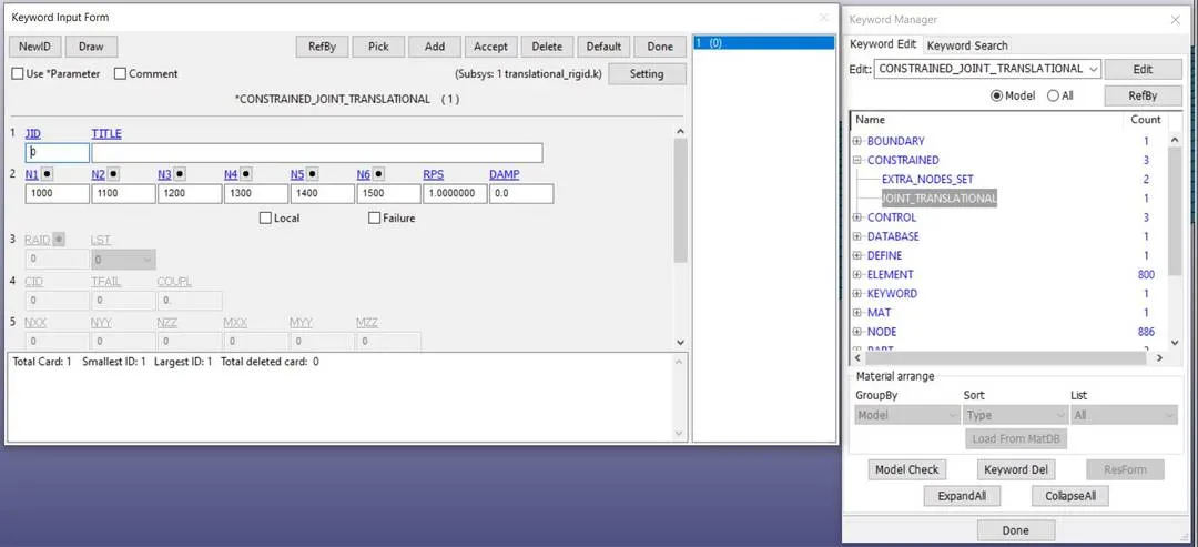
These nodes are assigned to translational joint by going to Constrained => Joint_Translational as shown below:

The nodes are assigned to respective parts in deformable joint as shown below using constrained nodal rigid bodies:

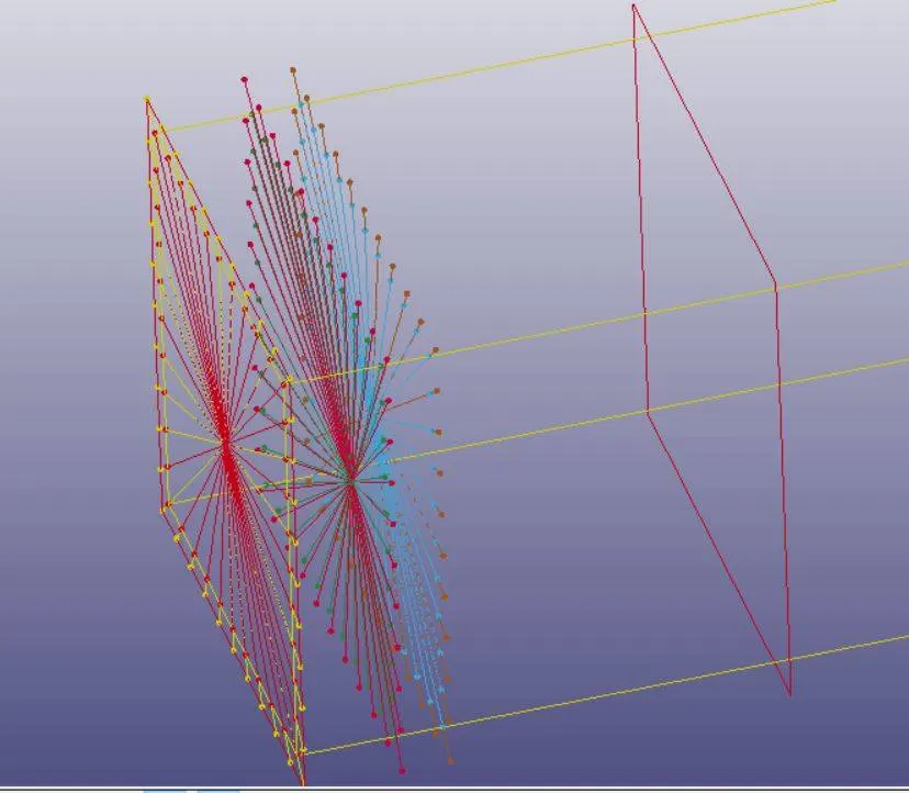
The boundary conditions for the deformable joints are shown below:

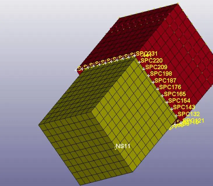
The yellow nodes are constrained in all degrees of freedom and the white node is given a translational degree of freedom. Implicit analysis is conducted to simulate the translational joint.

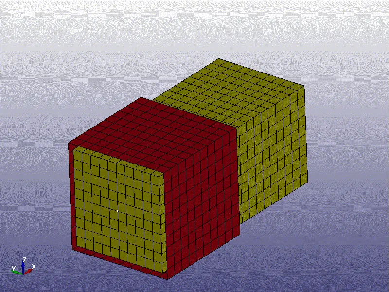
The result of rigid joint is shown below:

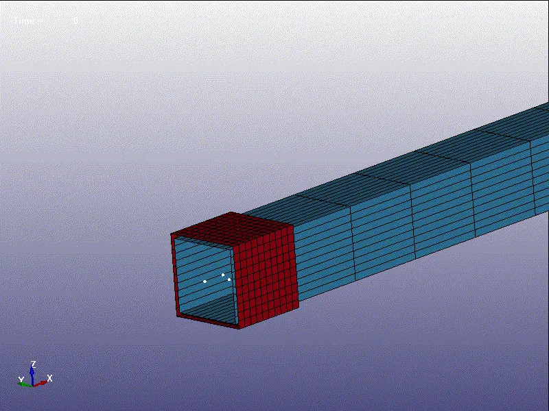
The result of deformable joint is shown below:

CONCLUSION: The four joints namely revolute, translational, spherical and cylindrical joints were successfully simulated and the results were demonstrated.