Week 11: FSAE Car Project

OBJECTIVE:

This is a simulation of the flow around an FSAE car with the following objectives:

• A baseline simulation of coarse mesh and publishing its results
• Refine the case for the following problem statement:

  ABCD Racing company is looking to perform Aero Simulations for their FSAE vehicle, and they have hired you to do the job. The suspension team wants a detailed report on the total downforce on individual components. They have two races this upcoming season.

  Race details are as follows

  Race-1

  • Racing track conditions - Lot of turns
  • Average lap speeds - 45kmph
  • 70% turns at 45 degrees
  • 20% turns at 80 degrees
  • 10% turns at 20 degrees

  Race-2

  • Racing track conditions - Straights
  • Average lap speed - 75kmph

BASELINE SIMULATION:

GEOMETRY:

We have an FSAE car STL file:

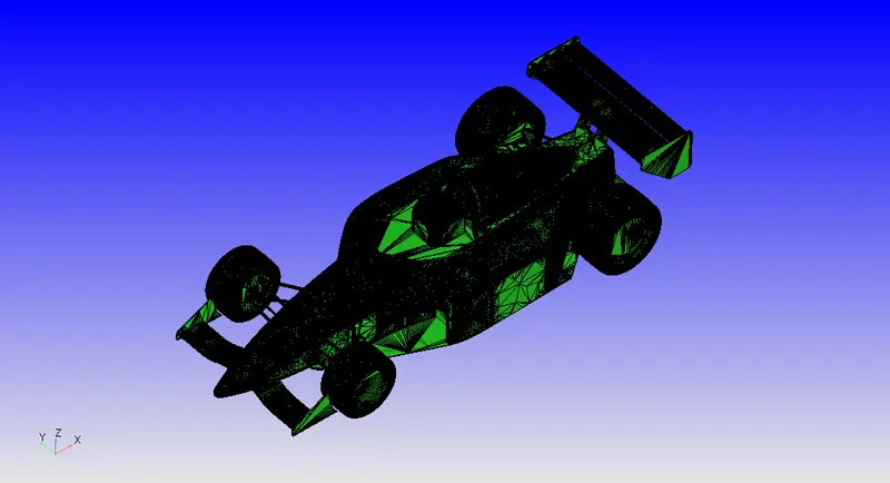
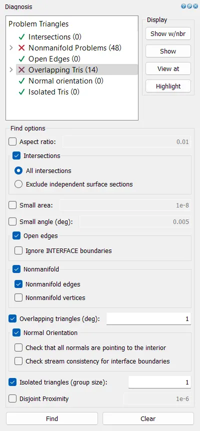
On diagnosis, It has following geometric errors which we will first fix:

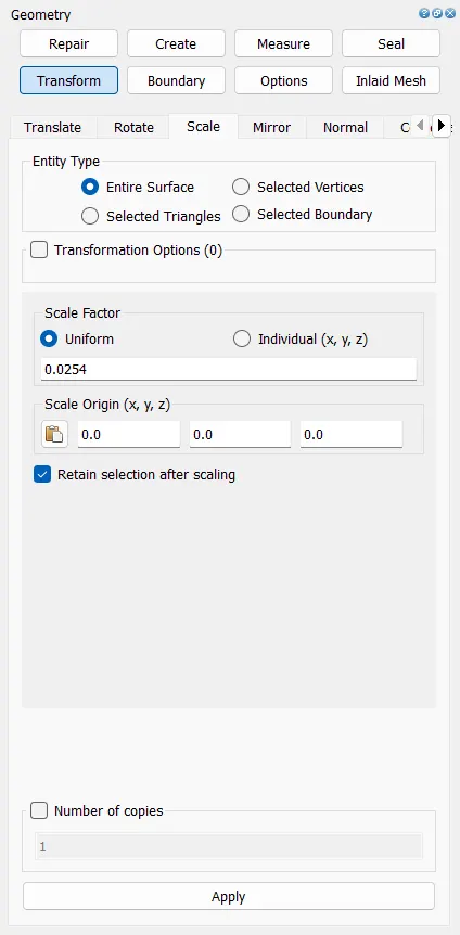
It was also mentioned that the STL file is in inches; hence we scale it since CONVERGE takes values in metres:

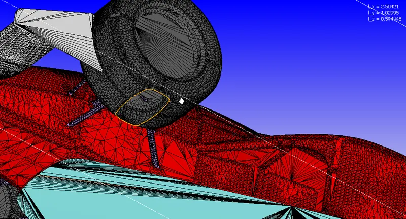
After finishing up with the preliminary fixes, we delete the flat surface from the bottom of the tires such that the bottom face of the virtual wind tunnel coincides with it creating a flat surface without creating geometrical errors:

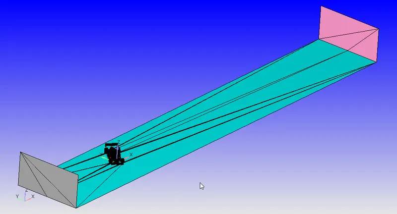
Wind Tunnel Dimensions:

The length of the car L = 2.5m, hence:

Distance between car nose and inlet = 3L
Distance from car nose to outlet = 10L
Distance from Flat tire to top = L
Distance from car nose to side wall = L

Total Length = 10L + 3L = 32.5m
Total Width = 2L = 5m
Total Height = L = 2.5m

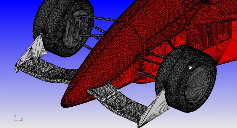
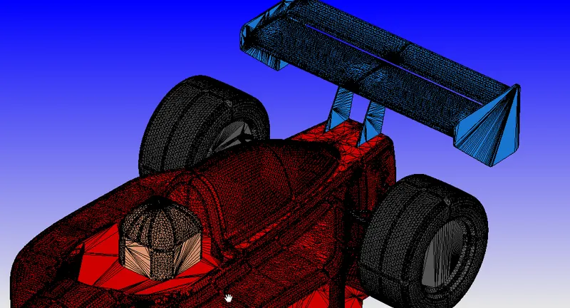
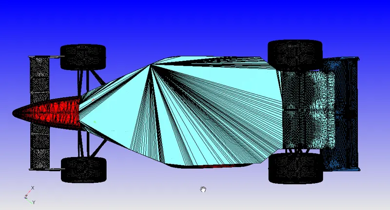
BOUNDARY FLAGGING:

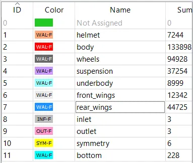
Car Components:

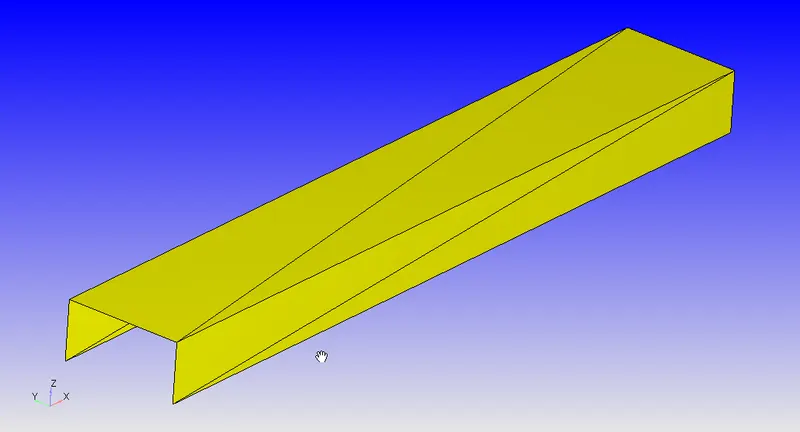
Symmetry Walls:

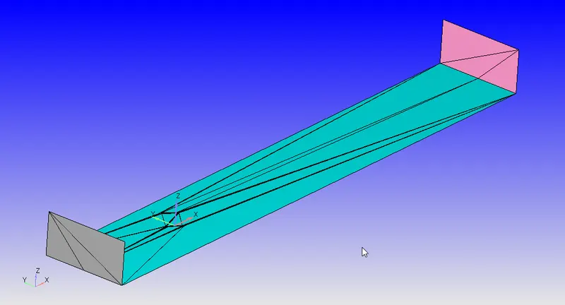
Inlet, Bottom and Outlet:

CASE SETUP:

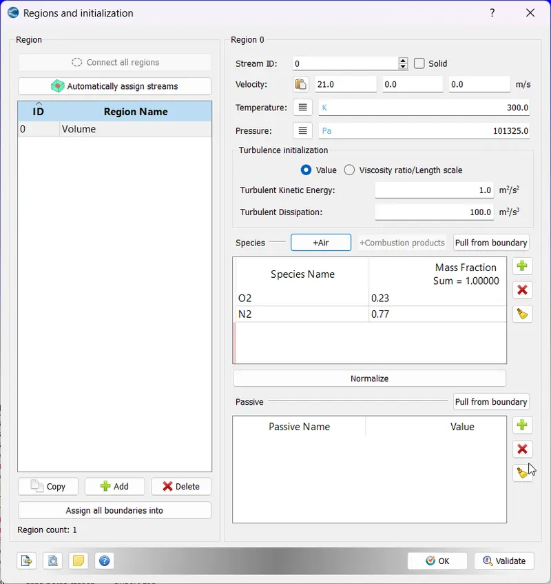
Initial Conditions:

Boundary Conditions:

*Except for Inlet, Outlet and Symmety walls, all boundaries follow the Law of the wall as a

Boundary condition*

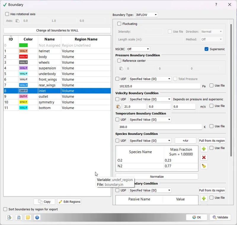
Inlet:

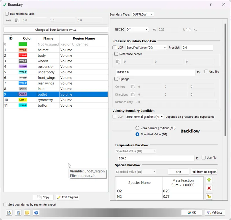
Outlet:

Solver Parameters:

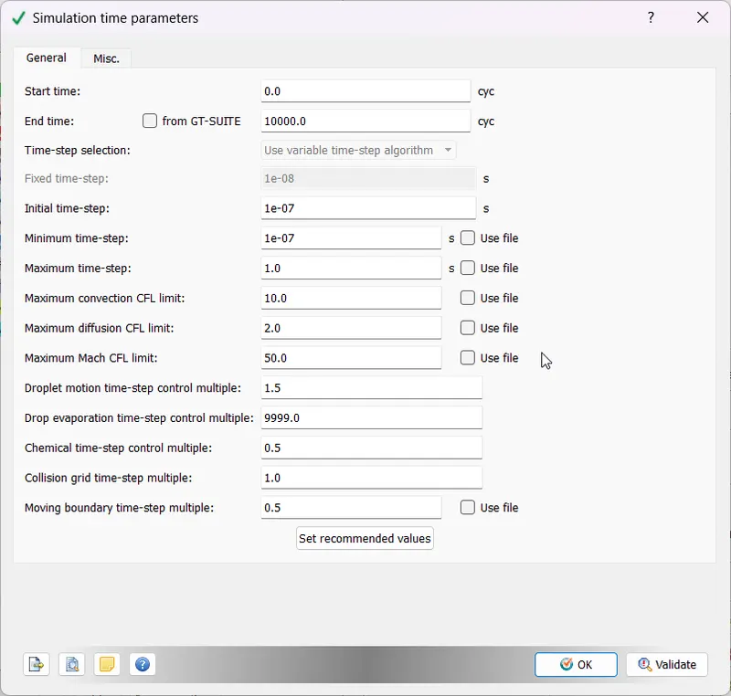
We are running a steady-state simulation using a density-based solver:

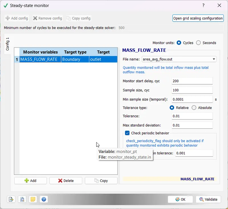
Steady-State Monitor:

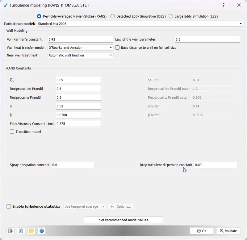
The turbulence model is a Standard k-omega model with automatic wall functions and default values:

Meshing:

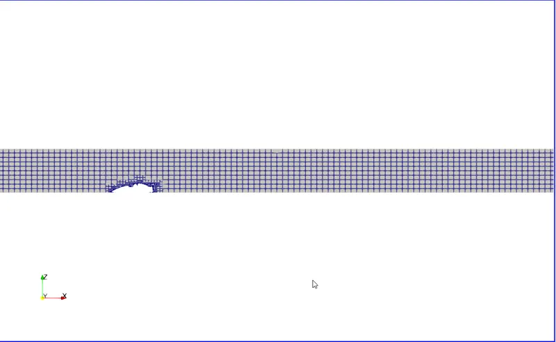
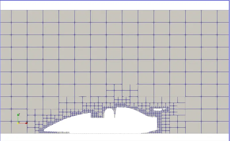
We use a coarse mesh of 0.1m and embedded mesh refinement for all vehicle boundaries of scale 3.

Output:

We are exporting y_plus and vorticity data along with standard variables and including the boundaries data using the "Boundaries Only" option for wall output.

RESULTS:

Mesh:

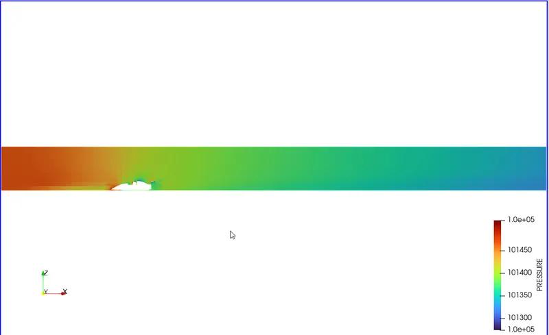
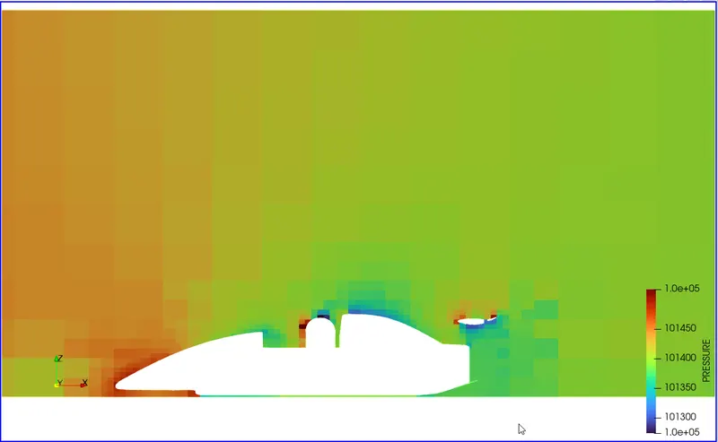
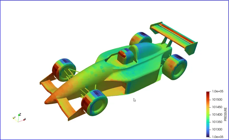
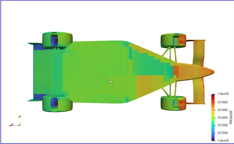
Pressure Contour:

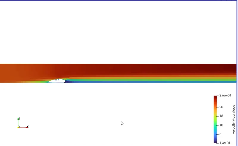
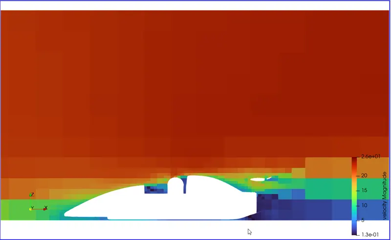
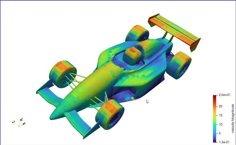
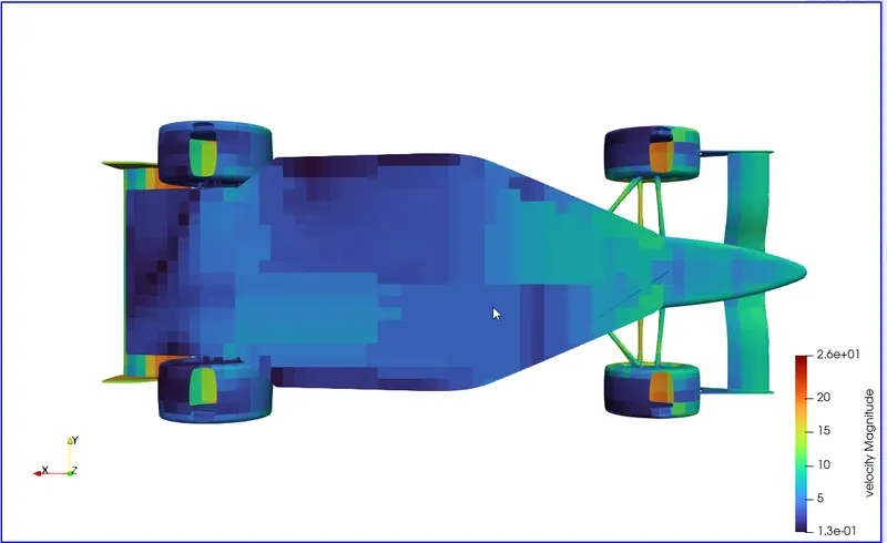
Velocity Contour:

RACE-1:

GEOMETRY:

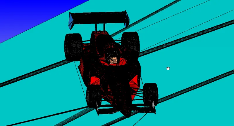
Since the track has a lot of turns, we will simulate the flow on the average angle of the turns. Given:

• 70% turns at 45 degrees
• 20% turns at 80 degrees
• 10% turns at 20 degrees

Average Turn Angle = 0.7*45 + 0.2*8 + 0.1*20 = 49.5 degrees

We will need to rotate the car components by 49.5 degrees:

CASE SETUP:

Initial Conditions:

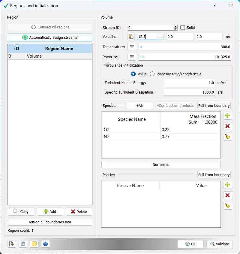
The velocity is given as 45 kmph = 12 m/s:

Boundary Conditions:

Same as the baseline setup, except for the inlet velocity, which is 12.5 m/s.

Solver Parameters:

We will run a transient simulation for detailed setups to better capture the wake region and account for the inaccuracies of the steady-state results. The Solver and turbulence model is the same as the baseline simulation.

Time Parameters:

We can guess the time required from the results of the Steady-state simulation:

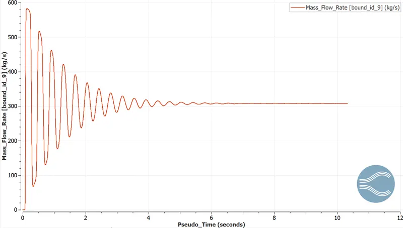
Around 8 seconds, the flow can be said to be converged. However, this is for an inlet velocity of 21 m/s.

Mathematically,

Flow throw time = 32.5/21 = 1.5 seconds

Usually, we set 5 times the flow throw time as the simulation end time; hence 7.5 seconds, which is analogous to our simulation results.

Similarly, for v = 12.5 s, Flow throw time = 2.6 seconds
Therefore, the Simulation end time `cong` 15 seconds.

Meshing:

Required wall distance:

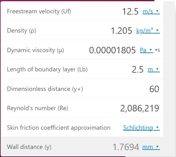
*yplus calculator; https://www.omnicalculator.com/physics/yplus

Hence, we can roughly take the wall distance `cong` 2 mm.

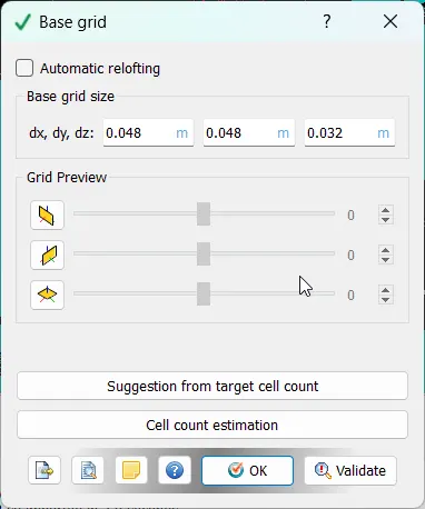
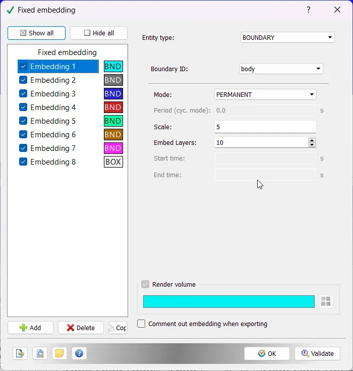
To balance scalability, CONVERGE recommends a maximum scale of 5 for mesh refinement. Hence we will use a `2^5 = 32mm` base mesh and use embedding with scale 5 for car components.

To further improve performance, we will increase the mesh size along the z and x directions by 50%:

Embedding for each component has similar parameters for scaling:

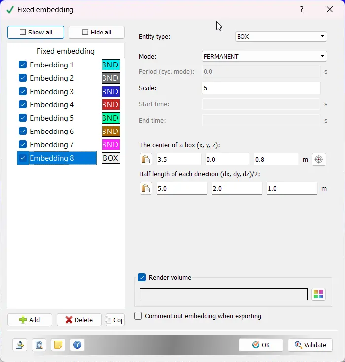
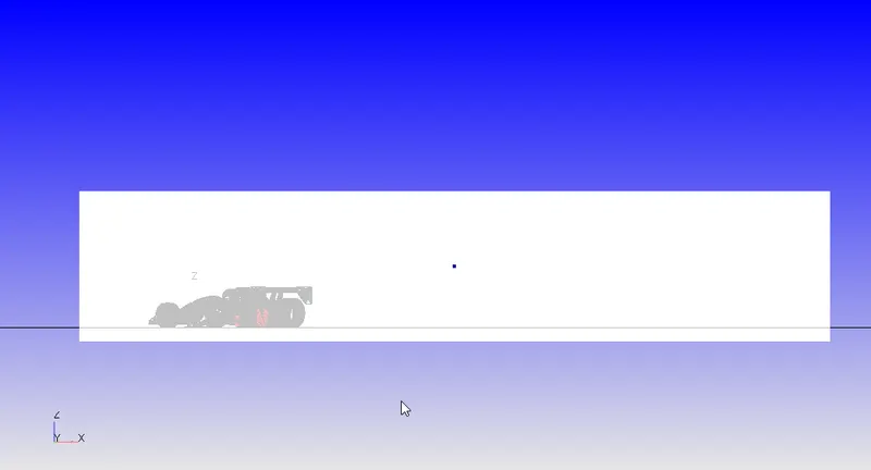
A box-type embedding is also added to improve the mesh in the wake region:

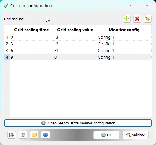
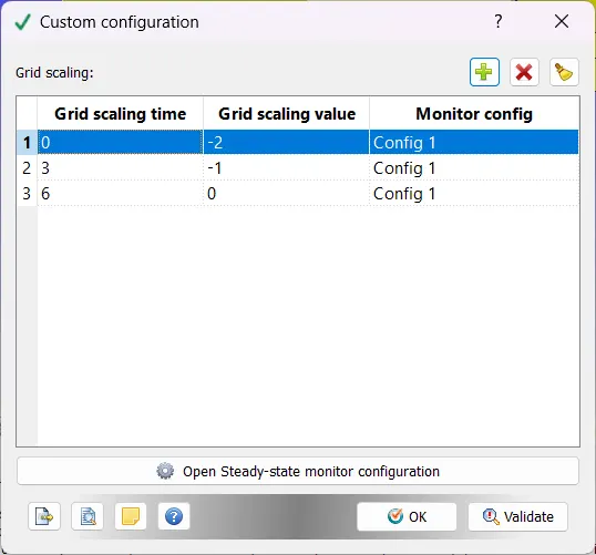
Lastly, we will add grid scaling to make our initial phase of simulation faster:

RACE-2:

GEOMETRY:

The geometry is the same as the baseline setup with no change.

BOUNDARY FLAGGING:

Boundaries are flagged the same as the other two cases.

CASE SETUP:

Given the velocity is 75 kmph = 21 m/s. The initial conditions will be the same as the baseline simulation

Boundary Conditions are also the same as baseline simulation.

Solver Parameters are the same as the RACE-1 case, transient density-based solver.

Time Parameters:

Using the analysis from the steady-state solution, we can use the simulation end time = 8 seconds.

Meshing:

Yplus value:

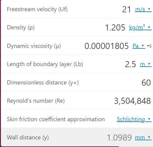
This gives us a minimal size for the first cell, which will require a lot of computational resources. We will use a higher value of yplus, around 80, for our first cell size `cong` 2mm.

We can then reuse the mesh settings from the RACE-1 case.

We will change the grid scaling:

CASE SETUPS: Setup Folder

CONCLUSIONS:

• Stead-state solutions are suitable for end results but produce wrong results when we want to observe a physical phenomenon. Since all physical phenomena are temporal, transient solutions offer more in-depth and accurate insights.
• Yplus is an essential parameter in determining the mesh size.
• Any simulation must be done in steps, verifying the results and slowly optimizing the process as you move towards higher accuracy. This helps in getting things done step by step, so we don't waste our time and computational power on a hasty simulation and end up with garbage data.