Week-11 Challenge: Braking

1. For a defined driving cycle, calculate the energy required for braking.

Solution:

Under the condition of braking, some amount of energy is required to do the same as that of energy required for accelerating the vehicle. Hence to calculate energy, we use the acceleration energy equarion,

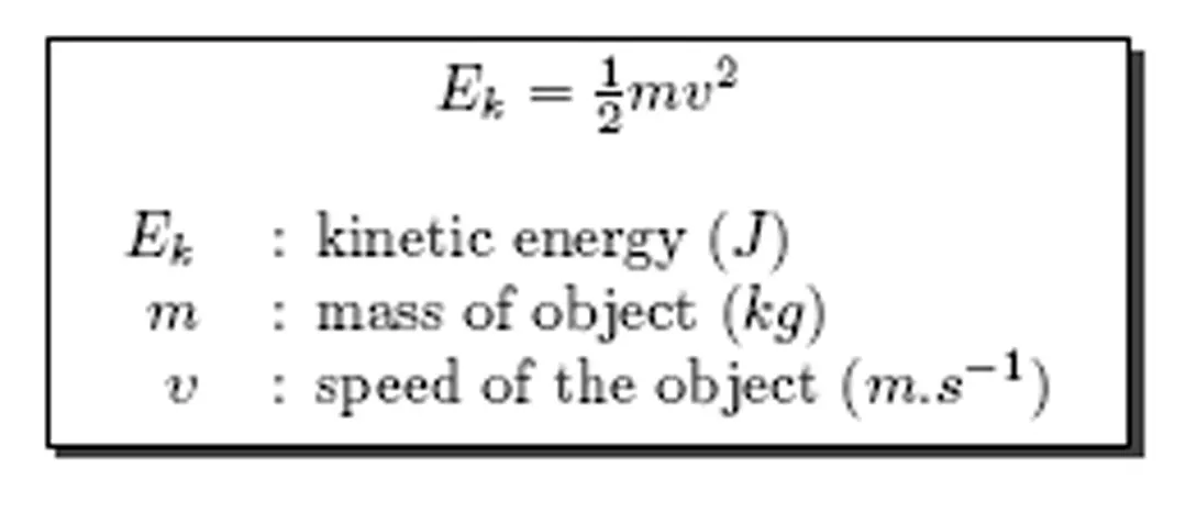
From the drive cycle, there are 4 different situations of decceleration of which the energy has to be calculated.

• First Braking : 24 - 15km/hr in 4 seconds
• Second Braking : 35 - 30km/hr in 1 second
• Third braking : 45 - 23 km/hr in 5 seconds
• Fourth braking : 62 - 5 km/hr in 7 seconds

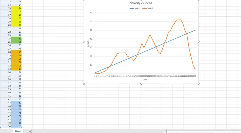
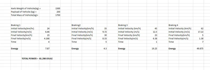
Total Braking energy required is 81.298 joules.

2. Why electric motor can’t develop braking torque at high speed similar to starting? How electric and mechanical brakes are coordinated?

Solution:

We can see that, at the time of accelerating vehicle at starting the maximum torque available motor is operating at constant torque region, in that motor will have maximum torque available, but as motor starts deccelerating motor characteristics are shifted towards braking region, in this we don’t have max torque available for braking as motor is already running at higher speed.

Due to this operation, electric motor can’t develop braking torque at high speed similar to starting

Electrical and mechanical braking systems can are coordinated by using Brake strategy subsystem

1) Serial Braking Strategy

2) Parallel Braking Strategy

Implementation of serial braking strategy

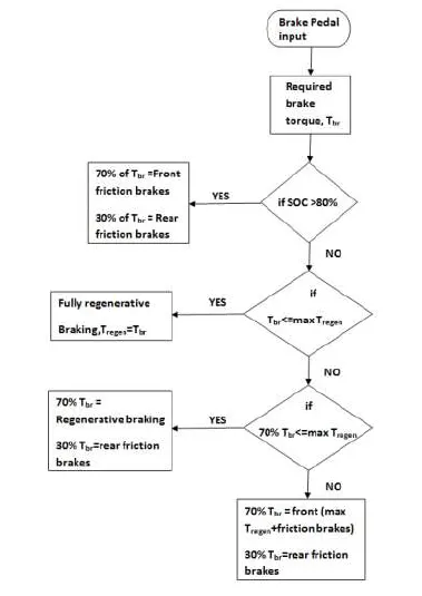
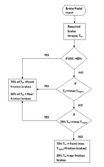
Once the brake pedal is pressed and depending on the level of depression, a brake torque is sent. Now this brake torque passes into the brake control strategy block. Here, firstly it is checked if battery state-of-charge is below 80% which is set as the maximum permissible level of charge. If that condition is satisfied, then the battery is recharged. The brake torque requested is compared to the maximum regenerative torque limit of the motor-generator. If the overall brake torque requested is less than or equal to the maximum regenerative torque, then the vehicle brakes purely on regenerative torque and the battery is charged. The amount of charge ultimately put in depends also on the motor-generator operation efficiency and the battery charging efficiency. If the overall brake torque requested is greater than what the motor-generator can provide, then the friction brakes kick-in. Now since the vehicle is front driven, it is checked if the total brake torque requested from front is less than or equal to maximum regenerative torque capability of motor-generator. If yes, then front braking is provided purely by regeneration and rear (non-driven axle) by friction. Once the total brake torque request increases further, then front friction brakes (driven axle) comes into play in combination with rear friction brakes and front regenerative braking, to satisfy the overall brake torque demand. This has been represented in a chart manner

Parallel Braking:-

Once the brake pedal is applied and a desired overall brake torque request is sent from the driver block. This brake torque on passing through the brake control strategy gets divided between regeneration and friction braking at all times. The strategy is so modeled with the comfort and brake pedal feel in mind. As a parallel regenerative braking is an add-on to the conventional systems, it is devoid of any integrated control. So to make the transition and co-performance of regenerative braking with friction smooth, it is assigned in such a way that, there is a clear division between the amount of brake torque that will be achieved from regeneration and friction braking. On application of brakes and in keeping with the design of the motor-generator, it is designed to operate generator in a constant generator torque region. Motor-generator can provide a maximum of 322 Nm of generator torque at or under the base speed. The generator is scaled such that the base speed of the generator corresponds to a velocity of 124 [kmph], which is the maximum speed limit on most highways. Hence regeneration works, as long as the vehicle is braking from a speed of under 124 [kmph] and the requested brake torque on the front driven wheels, after the front-rear brake split is greater than or equal to maximum generator torque. If that condition is satised, then regenerative and friction braking operates in tandem else it’s just the friction brakes at the driven and non-driven axle. This has been represented in a ow chart manner in the g.1.5.

3. Make a MATLAB program which plots contour of given motor speed, torque and efficiency values. Attach the code as a .m file attach a screenshot of all the plots.

Solution :

clear all
close all
clc

x = linspace(1,1000) %defining speed
y = linspace(1,250)  %defining torque

%Motor loss constants

kc = 0.2             %copper losses
ki = 0.08            %iron losses
kw = 0.00001         %windage losses
cml = 400            %constant motor losses

[X Y] = meshgrid(x,y);   %meshgrid command to plot 3D graph.

output_power = (X.*Y)    %ouputpower = speed * torque

B = (Y.^2)*kc            %Copper loss
C = X*ki                 %Iron loss
D = (X.^3)*kw            %Windage loss



input_power = output_power+B+C+D+cml;  % formula for input power

Z = output_power./input_power;         %efficiency of motor
V = [0.5,0.6,0.7,0.8,0.9,0.10]         %efficiencies for which the graph is plot

figure(1)
contour(X,Y,Z);                        %contour command to plot the graph
figure(2)
plot3(X,Y,Z);
hold on

v=[3000,5000];
contour(X,Y,output_power,v);

Explanation :

• Here x is defined as the speed and we use 'linspace' command to specify 1000 values for the speed parameter.
• Here y is defined as the torque and we use the 'linspace' command to specify 250 values for this parameter.
• All the motor constants are defined
• Kc is the copper losses which has a value of 0.2
• ki is the iron losses which has a value of 0.08
• Kw is the winding loss which has a value of 0.00001.
• The cml is constant motor loss which is 400.
• Then we use the meshgrid command to make an array of x and y coordinates to plot the 3D graph in the form of X and Y.
• The output power is given by the value of speed multiplied by torque.
• The copper loss is calculated with a square term of x multiplied by the copper loss constant.
• The iron loss has an x term multiplied by loss constant.
• The winding loss has an cubic term of x gained by the loss constant.
• Input power is calculated by the formula = output power + B + C + D + cml
• Z is the efficiency of the motor can be calculated output power/input power.
• And the v is a variable used to define the efficiencies to plot the contour curve.
• plot3 command is used to get a real time plot of the values of the graph.
• Contour creates a contour plot containing the isolines of matrix Z, where Z contains height values on the x-y plane. MATLAB automatically selects the contour lines to display. The column and row indices of Z are the x and y coordinates in the plane, respectively.

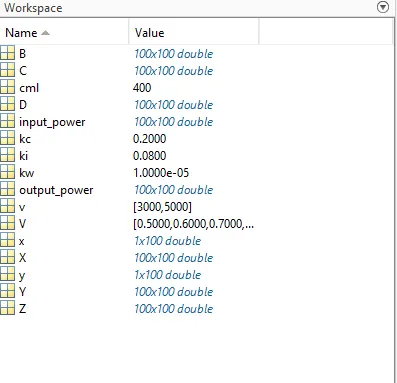
• All the values found during the calculation is shown in workspace.
• All the values are in array of 100*100 matrix.
• The values of input power and z are found out.

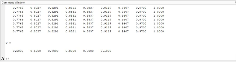
• An array of 100 columns are obtained as result.
• The input efficiencies are specific.

Result :

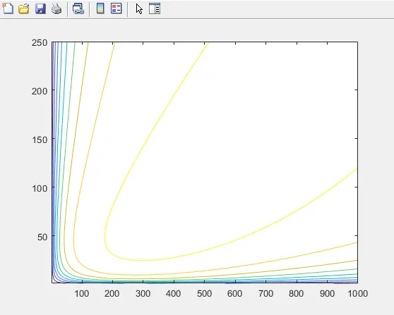
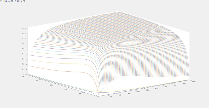
• Figure 1 shows the top view of the contour plot.
• Figure 2 shows the 3D plot of the graph.
• We can understand from the result that speed is inversely proportional to torque.
• When speed increases the torque goes on decreasing and vice-versa.
• We can see that when the maximum concentration is at the centre.