Week-11 Challenge: Braking

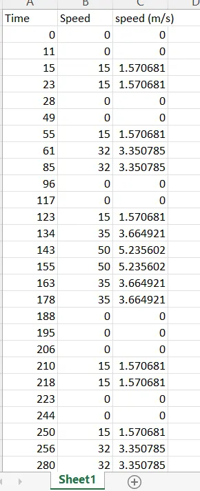
1. NEDC is the driving cycle selected. The values of speed and time is entered in excel. This is then loaded in MATLAB workspace and program is executed to calculate the braking energy .

m=1000;
t=drivecycle(:,1);
v=drivecycle(:,3);
for i=1:(length(drivecycle)-1);
   if v(i)>v(i+1)
       BE(i)= 0.5*m*(v(i)-v(i+1))^2;
   end 
end
fprintf('total brake energy is %d', sum(BE))
%figure (1); 
%plot(2,1,1);
plot (t, v, 'color','r');
xlabel( 'Time(s)');
ylabel('Energy(J)');
title('Braking Energy')

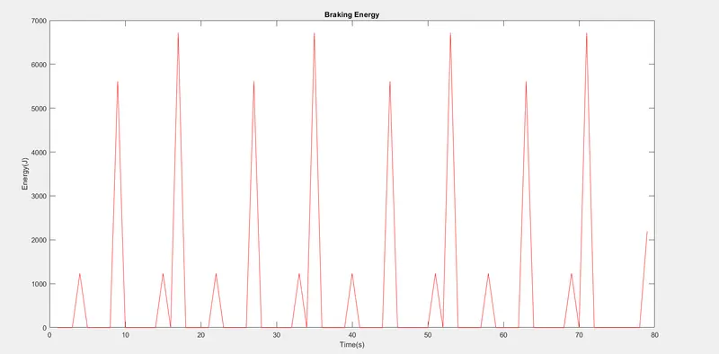
total brake energy is 6.137990e+04>> 

Energy required is calculated using formula BE=0.5*m*(v(i)-v(i+1))^2

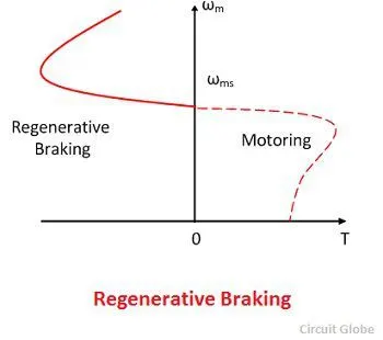
2. At starting , back emf of the motor is low hence input current is allowed to rise. It is mainly used to increase the kinectic energy of the load. But after attaining the rated speed, back emf of the motor is high, therefore current cannot be increased beyond that limit. ie operation beyond rated speed always happens with comprimse in the torque performance. Also during braking operation the direction of rotation of motor is in the reverse direction which limits its operation.

Electrical and mechanical brakes

The desirable braking system of vehicle is that it must be stopped or even reduce the speed when brakes are applied. If the charging limit of the battery is less than the regenerative power requirement then mechanical brakes also comes in picture. efficient brake control strategies must be defined in such as way to ensure good braking performance as well as recovering maximum energy during regeneration.Electric driven brake combines both mechanical and electrical brake where at low speed regeneration is used and at high speed combination of mechanical and regeneration is used.

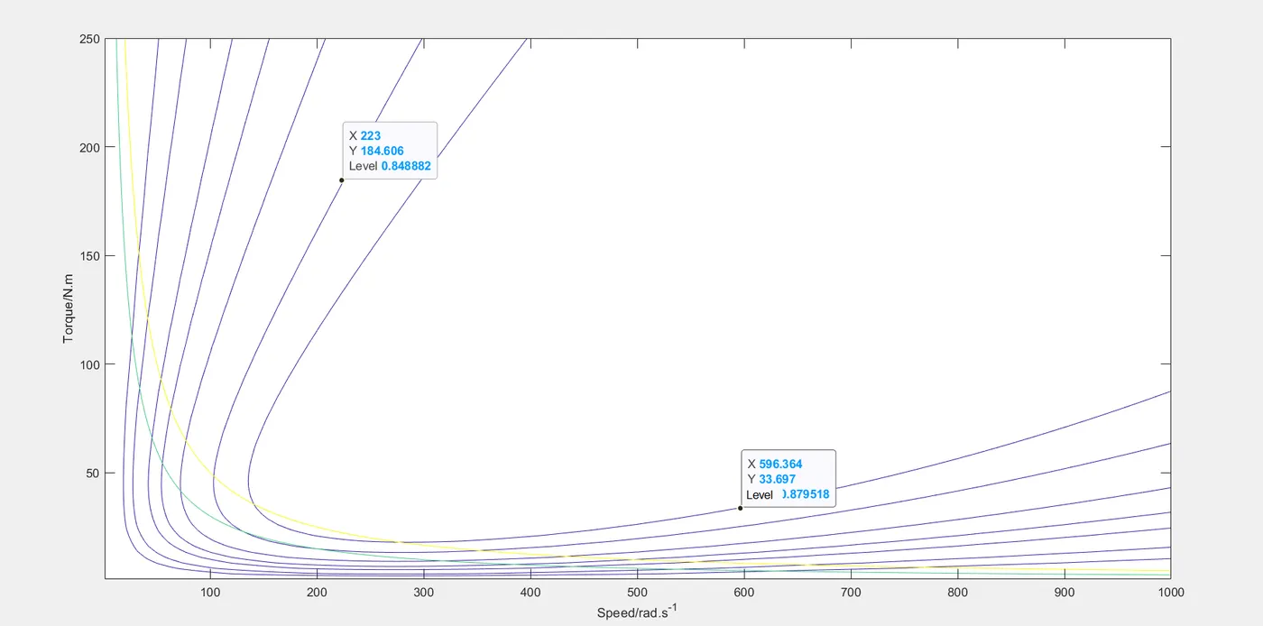
3.The mATLAB program for efficiency plot is shown.

lear all
clc
x=linspace(1,1000);% speed, N.B. rad/s NOT rpm
y=linspace(1,250); % 0 to 40 N.m

% Allocate motor loss constants.
kc=0.2; % For copper losses
ki=0.008; % For iron losses
kw=0.00001;; % For windage losses
ConL=400; % For constant motor losses

% Now make mesh
[X,Y]=meshgrid(x,y);
Outputpower=(X.*Y); % Torque x speed = power
B=(Y.^2)*kc; % Copper losses
C=X*ki; % Iron losses
D=(X.^3)*kw; % Windage losses

Inputpower = Outputpower + B + C + D + ConL;
Z = Outputpower./Inputpower;

% We now set the efficiencies for which a contour
% will be plotted.
V=[0.5,0.6,0.7,0.75,0.8,0.85,0.88];
box off
grid off
contour(X,Y,Z,V);
xlabel('Speed/rad.s^-^1'), ylabel('Torque/N.m');
hold on
% Now plot a contour of the power output
% The array Output Power has
% already been calculated. We draw contours at
% 3 and 5 kW.
V=[3000,5000];
contour(X,Y,Outputpower,V);