Week-11 Challenge: Braking

1)Aim:

To calculate the brake energy for a drive cycle.

Explanation:

A brake is a mechanical device that inhibits motion by absorbing energy from a moving system.It is used for slowing or stopping a moving vehicle, wheel, axle, or to prevent its motion, most often accomplished by means of friction.A moving vehicle possesses kinetic energy and to stop the vehicle, the energy of the moving vehicle has to be converted into another form. The friction brake system in a conventional vehicle dissipates kinetic energy in the form of heat energy. If the complete kinetic energy is transformed into another form of energy, then the vehicle stops. As a result of friction, heat energy is being generated in the braking system when the vehicle brakes.

In the case of Electic Vehicles, when we accelerate the vehicle, energy in the battery flows to the electric machine to drive it. The energy required to move the vehicle is taken from the battery. The actuator pedal is released to slow down the vehicle and when it is completely released, the power flow to the motor from the battery stops. As a result, the vehicle starts to decelerate due to the aerodynamic drag, rolling friction, and other forces that oppose the movement of the vehicle. But those friction forces are not sufficient to stop the vehicle and hydraulic brakes are also applied. So, the kinetic energy is converted to heat energy at the brake, and the vehicle stops.

Formula:

Brake Energy = `1/2*m*(V_f-V_i)^2`

where

m = Mass of the vehicle

Vf= Final speed of the vehicle

Vi= Initial Speed of the vehicle

Code:

clear all;
close all;
mass=input("Enter the Mass of the vehicle");
drive_cycle=xlsread('Drivecycle-ftp75');
time=drive_cycle(:,1);
speed=drive_cycle(:,2);
for i=1:(length(speed)-1)
    if speed(i)>speed(i+1)
        br(i)=0.5*mass*(speed(i)-speed(i-1))^2;
    end
end
fprintf("Total brake energy is %d kJ",sum(br)/1000);
subplot(2,1,1);
plot(time,speed);
xlabel("time");
ylabel("speed");
title("drive cycle");
hold on;
subplot(2,1,2);
plot(br);
ylabel("Brake energy");
title("Brake energy");

Explanation:

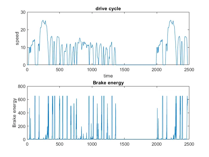
The brake energy is calculated for the drive cycle of FTP-75 cycle.The drive cycle is load using xlsread option. The mass of the vehicle is inputted via command window and using for loop the brake energy is calculated.

Result:

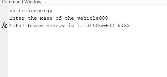
The mass of the vehicle is 600 kg and brake energy calculated for the driving cycle is 1.130KJ and drive cycle and brake energy is plotted below.

2)Aim:

To explain about the braking torque at high speed similar to starting and explain the electric and mechanical brakes are coordinated.

Explanation:

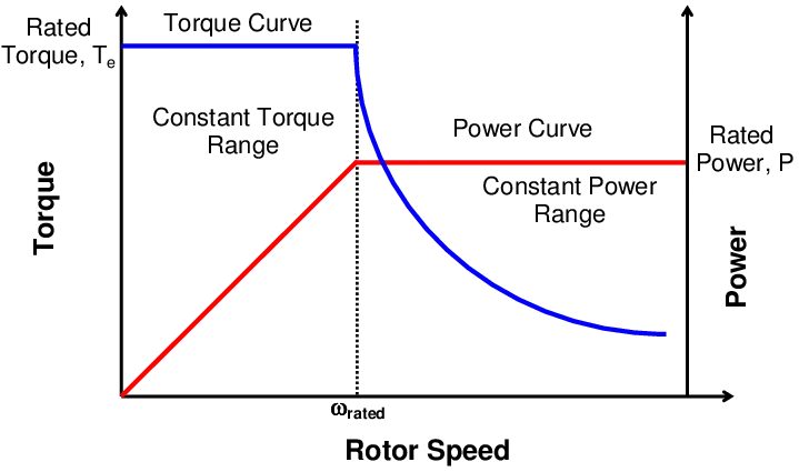
During the Acceleration condition, the motor operates in the 1st region where the torque and speed are positive and till the speed reaches rated values it operates on the constant torque region and after the rated value of speed, it operates in the constant power region. During braking or deceleration conditions, the motor operates in the 2nd region where the torque and speed are positive and negative respectively. Its mirror image of acceleration plot. Its operation above base speed and field weakening region, the peak of acceleration torque is greater than braking torque.

Electrical and Mechanical brake coordination:

There two types of coordination techniques are used.

Series:

Brakes will be applied one after another. In case regenerative brakes used for some time then mechanical brakes used after the regenerative braking.

Parallel:

Both Brakes are applied at the same time. In this case, regenerative braking and mechanical braking are applied at the same time.

Electric Driven Intelligent Braking:

EVs and hybrid vehicles use regenerative braking, which utilizes the motor to convert the kinetic energy during deceleration into electrical energy. With energy regeneration, an EV is able to run on less electricity and a hybrid vehicle on less fuel. The EDIB (Electric Driven Intelligent Brake) allows and controls optimization of the regenerative brake and regular friction brake (hydraulic brake).

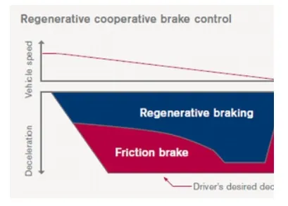
EDIB (Electric Driven Intelligent Brake) controls the regenerative brake and friction brake to support both of these requirements. Further, it also controls the reactive force from the pedal in order to unify the feeling when stepping down on the pedal and the sense of deceleration.

3)Aim:

To write a Matlab program to plots the contour of given motor speed, torque and efficiency values.

Explanation:

Copper loss:

Copper loss is due to the resistance of the wire in the primary and secondary windings and the current flowing through them. These losses can be reduced by using wire with a large cross-sectional area in the manufacturing of the coils.

Iron loss:

Also called core losses, these are associated losses in the magnetic paths of the motor. They are usually characterized as watt loss per mass. Different steels have different characteristics that impact these losses. In order to understand iron losses better, we can further divide them into hysteresis losses and eddy current losses.

• Hysteresis losses are due to the changing polarity of the flux in the steel core. Hysteresis losses are affected by both the ability of the material to change polarity easily and by the total flux density in the steel.
• Eddy current losses are circulating currents induced in the steel core by the changing polarity of the flux. Eddy current losses are affected by the total flux density, the frequency at which the polarity of the flux changes and the area available for eddy currents to flow. Motor designs use laminated cores of steel to reduce the area available for the eddy currents to flow because the electrons are unable to jump from lamination to lamination.

Windage loss:

Windage loss combines losses from the rotor spinning in the air that creates drag and those from cooling fans used on the motor, along with friction losses in the bearings.

Forumla:

Efficiency = Output power / Input power

Input power = Output power + losses

losses = Copper loss + Iron loss + Windage loss + constant loss

losses = `K_c*T^2 + K_i * omega + K_w*omega^3 + c`

where

T = Torque in N-m;

`omega =`speed in m/s

c is constant loss

Output power = Speed * torque.

Code:

speed=linspace(1,1000);
torque=linspace(1,300);
kc=0.2;
ki=0.008;
kw=0.00001;
[X,Y]=meshgrid(speed,torque);
c=20;
outputpower=(X.*Y);
copperloss=(Y.^2)*kc;
ironloss=X*ki;
windageloss=(X.^3)*kw;
Inputpower=outputpower+copperloss+ironloss+windageloss+c;
z=outputpower./Inputpower;
v=[0.70,0.80,0.85,0.90,0.95,0.99];
box off;
grid off;
contour(X,Y,z,v);
xlabel('speed');
ylabel('torque');
title("Contour plot");

Result:

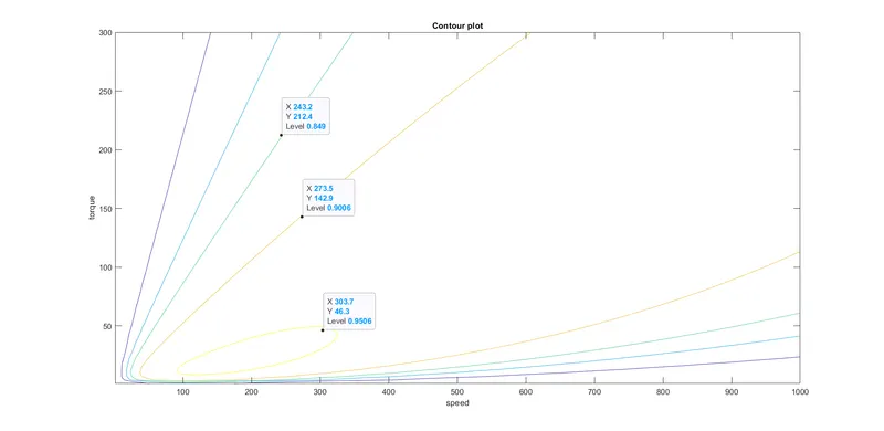
From the contour plot,the highest efficieny arises in the innermost of the contour plot and this efficieny decreases as contour moves from innermost ot outermost contour . From the plot the ineermost contour is 95% and as plot moves outermost it decreases as from 95%.