Week 11- Broadband Noise modelling over Ahmed body

Aim:

1. Describe Ahmed's body and its importance.
2. Setup the domain and setup assuming body is travelling at 110 kmph
3. Run the setup till convergence and plot for static pressure and coefficient of drag and lift to check for convergence
4. Turn on Broadband- modelling and detail the acoustic field study over Ahmed body.

Ahmed Body & its Importance:

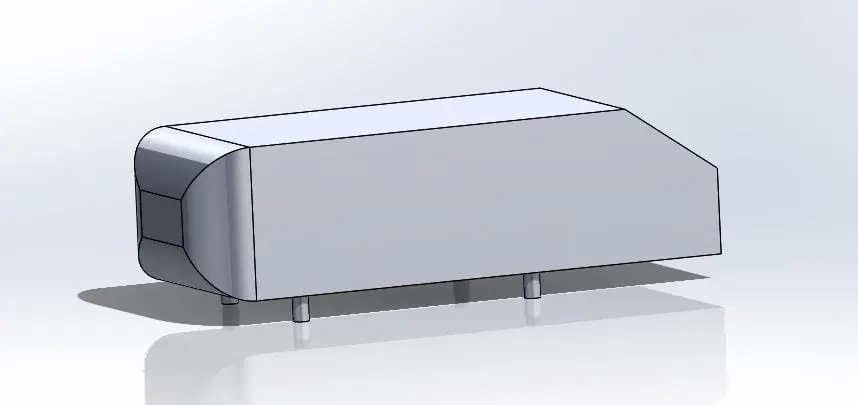
• Ahmed body is a geometrical shape which was first created by Ahmed and Ramm in 1984, in order to study the aerodynamic flow characteristics and validate the result obtained.
• Ahmed body was the generic car body which is used to capture the essential flow characteristics that are relevant to bodies in the automobile industry.
• This model is also used to describe the turbulent flow field around a car like geometry.
• Once the numerical model is validated, it is used to design new models of the car.

Aerodynamic Acoustics Model:

Many sounds that are technologically important in industrial applications are generated by and propagated in fluid flows. The phenomena associated with sounds can therefore be understood and analyzed in the general framework of fluid dynamics.

Challenges faced:

• Numerically predicting sound waves stems from the well-recognized fact that sounds have much lower energy than fluid flows, typically by several orders of magnitude. This poses a great challenge to the computation of sounds in terms of difficulty of numerically resolving sound waves, especially when one is interested in predicting sound propagation to the far field.
• The difficulty of predicting the very flow phenomena (e.g., turbulence) in the near field that are responsible for generating sounds.

computing aerodynamically generated noise is done using three approaches they are as follows.

• Direct Method
• Integral Method Based on Acoustic Analogy
• Broadband Noise Source Models

1. Direct Method:
   • Both generation and propagation of sound waves are directly computed by solving the appropriate fluid dynamics equations. Prediction of sound waves always requires time-accurate solutions to the governing equations. Furthermore, in most practical applications of the direct method, one has to employ governing equations that are capable of modeling viscous and turbulence effects, such as unsteady Navier-Stokes equations (i.e., DNS), RANS equations, and filtered equations used in DES and LES.
   • The direct method is thus computationally difficult and expensive, as it requires highly accurate numerics, very fine computational meshes all the way to receivers, and acoustically non-reflecting boundary conditions.
   • The computational cost becomes prohibitive when sound is to be predicted in the far field (e.g., hundreds of chord-lengths in the case of an airfoil). The direct method becomes feasible when receivers are in the near field (e.g., cabin noise).
   • In many such situations involving near field sound (or pseudo-sounds for that matter) are predominantly due to local hydrodynamic pressure which can be predicted with a reasonable cost and accuracy.
2. Integral Method Based on Acoustic Analogy:
   • In this approach, the near-field flow obtained from appropriate governing equations such as unsteady RANS equations, DES, or LES are used to predict the sound with the aid of analytically derived integral solutions to wave equations. The acoustic analogy essentially decouples the propagation of sound from its generation, allowing one to separate the flow solution process from the acoustics analysis.
   • The FW-H formulation adopts the most general form of Lighthill’s acoustic analogy, and is capable of predicting sound generated by equivalent acoustic sources.
   • One important limitation with integral FW-H formulation is that it is applicable only to predicting the propagation of sound toward free space. Thus, while the model can be legitimately used to predict farfield noise due to external aerodynamic flows, such as the flows around ground vehicles and aircraft, it cannot be used for predicting the noise propagation inside ducts or wall-enclosed space.
3. Broadband Noise Source Model:
   • Many practical applications involving turbulent flows, noise does not have any distinct tones, and the sound energy is continuously distributed over a broad range of frequencies. In those situations involving broadband noise, statistical turbulence quantities readily computable from RANS equations can be utilized, in conjunction with semi-empirical correlations and Lighthill’s acoustic analogy.
   • Unlike the direct method and the FW-H integral method, the broadband noise source models do not require transient solutions to any governing fluid dynamics equations. All source models require what typical RANS models would provide, such as the mean velocity field, turbulent kinetic energy and the dissipation rate. Therefore, the use of broadband noise source models requires the least computational resource.

Geometry:

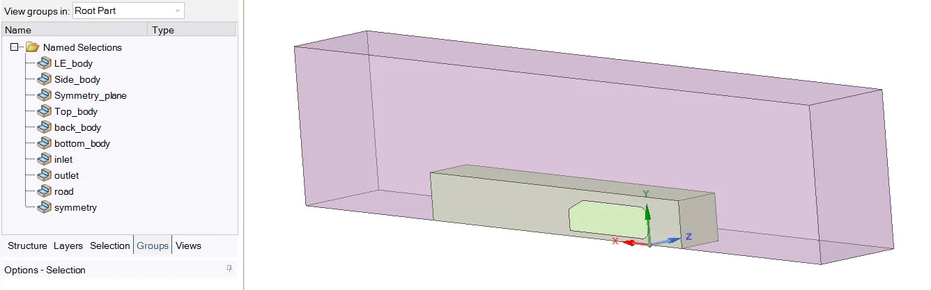
Import the ahmed body model and open in space claim to check the naming conventions.

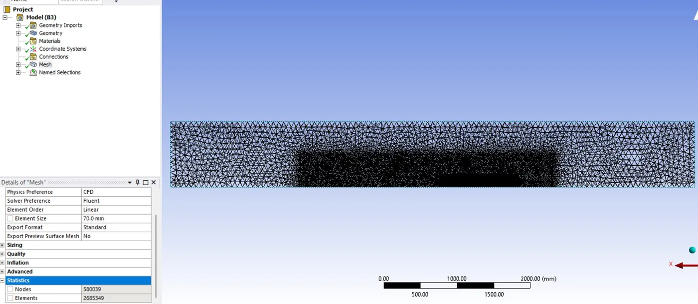
Mesh: ( Inorder to reduce the computational load element size and inflation layer size has been increased but still result obtained is not deviated much)

• Element size of the model is kept to be 70mm

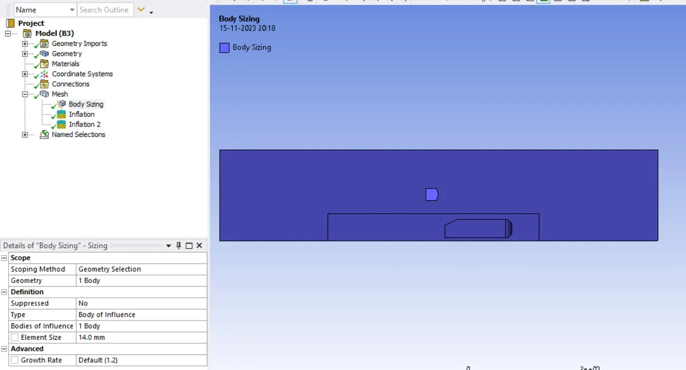
• Body sizing: Refined mesh is assumed at the closed domain of the ahmed body, which is ad possible by using body sizing the closed domain is assumed to be 14mm, whereas the overall domain is assumed to be at 70mm element size.

• Road Inflation: select the domain on which the inflation needs to be absorbed then select the road face on which the inflation is required. First aspect ratio is assumed to be 5 with maximum of 5 layers and growth rate of 1.2

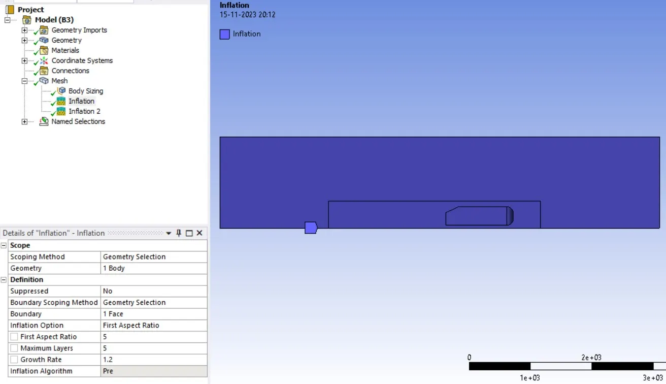
• Ahmed Body Inflation: select the domain on which the inflation needs to be absorbed then select the Ahmed Body on which the inflation is required. First layer height is 0.01mm, maximum 28 layer with 1.2 growth rate.

from the Y+ calculation:

• Desired Y+=1
• Free Stream Velocity = 31m/s (approx)
• Density = 1.225 Kg/m3
• Viscosity = 1.8 x 10^-5 Kg/ms
• Characteristics length = 3.7 x 0.297= 1.0989
• Re = 2271060
• First Cell Height = 0.01mm

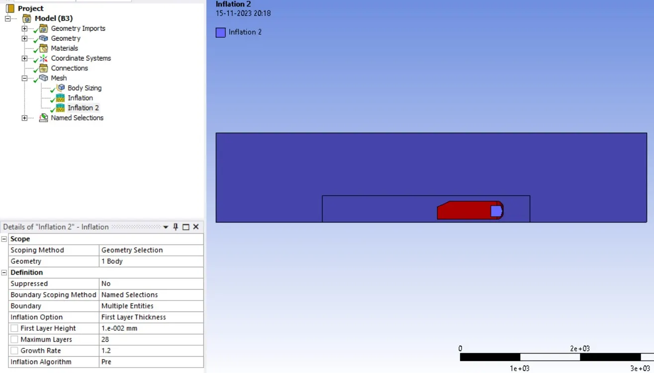
• Inflation layers is essential to calculate the acoustic, drag and lift parameters near wall more accurately. Further, check the quality of the mesh so that we do not encounter any over inflated values.

Element Quality

Skewness

Aspect Ratio

Orthagonality

Simulation Setup:

• General setting: Pressure Based, Steady state, absolute velocity formulation. Enable to solve energy equation as well
• Viscous model: K-Epsilon, Realizable, Enhanced wall treatment & enable production limiter.
• Cell zone: Fluid Domain (Air)
• Boundaries:
  • Ahmed body walls are given stationary wall boundary condition
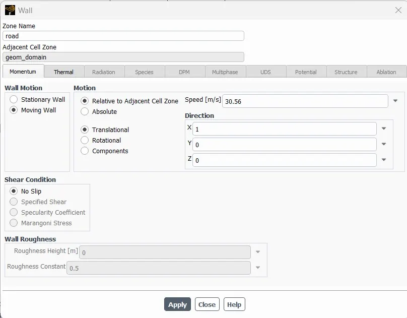
  • Road is given moving wall boundary condition
• 
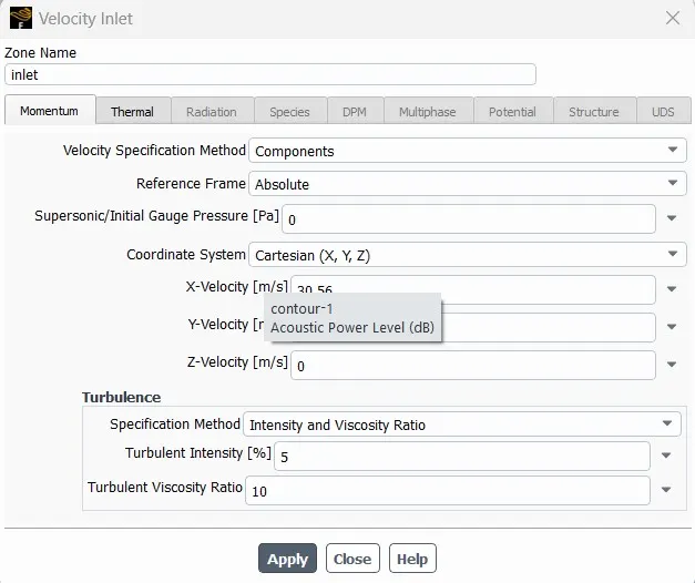
  • Inlet is given velocity boundary condition

• 
  • Outlet is given pressure boundary condition
  • Symmetry plane & symmetry is given symmetry boundary condition.

• Reference values: Compute from inlet and calculate the cross section area of ahmed body and rewrite it.

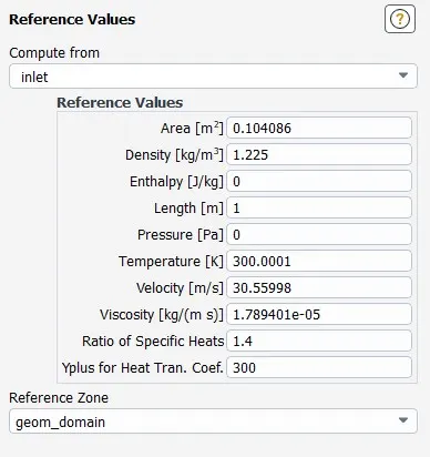
• Method: use pressure velocity coupling method and enable second order upwind method for all the equation.
• Control: enable 10 as the flow courant number
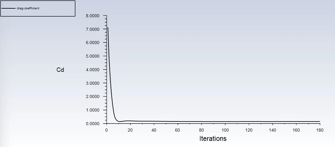
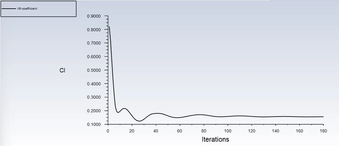
• Report definition: In order to check the convergence criteria, we have to create drag and lift coefficient plot over the ahmed body wall apart from the residual plot.
• Initialization: we have enabled standard initialization method.
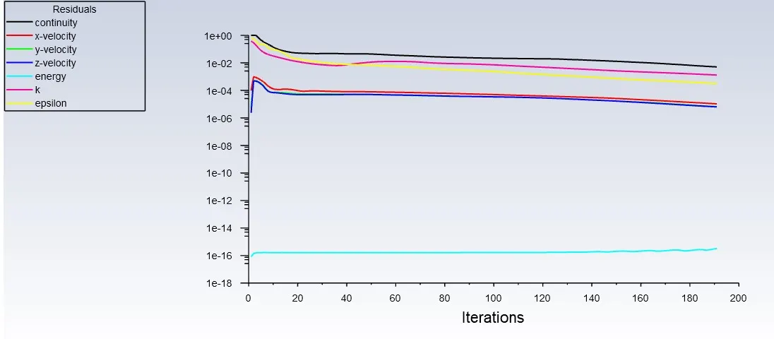
• Run calculation: we have run the simulation for 190 iteration. By then the residual, drag and lift coefficient plot have converged and any further solving will not result any drastic change in result.
• Acoustic Model: Once the usual simulation is run, Enable the acoustic model for 100 number of realization.

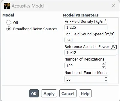
Post Processing: (Result is converged by 190 iteration so the simulation was stopped)

• Residual

• Coefficient of Drag

• Coefficient of Lift

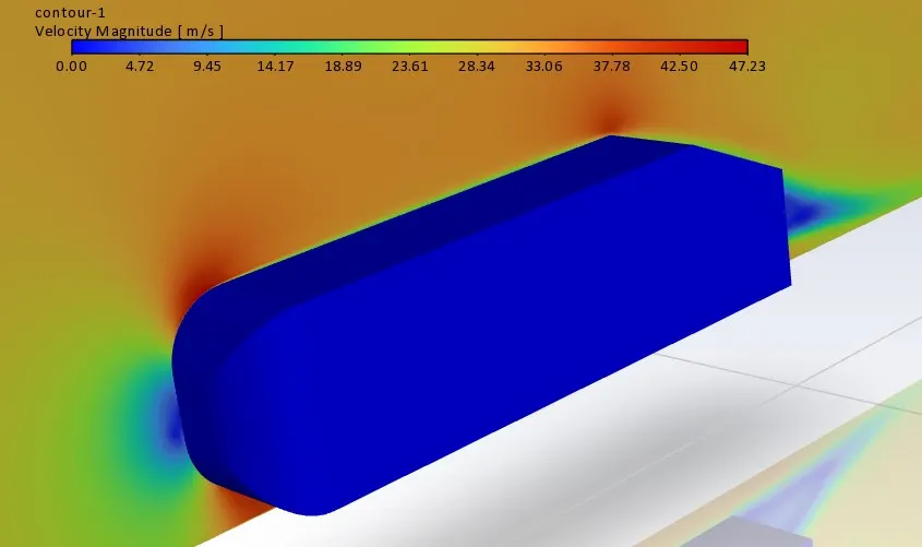
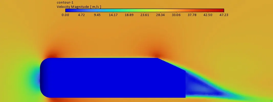
• Velocity contour

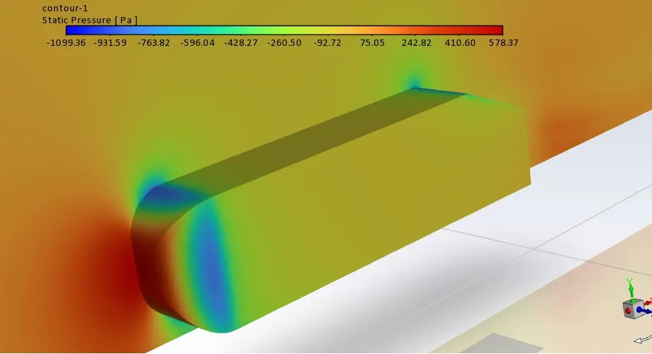
• Static pressure contour

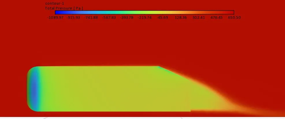
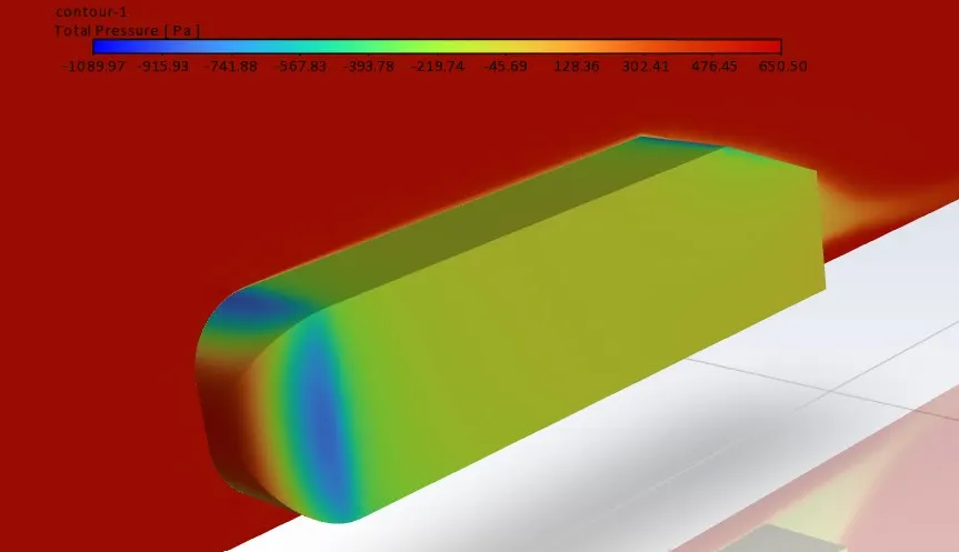
• Total pressure contour

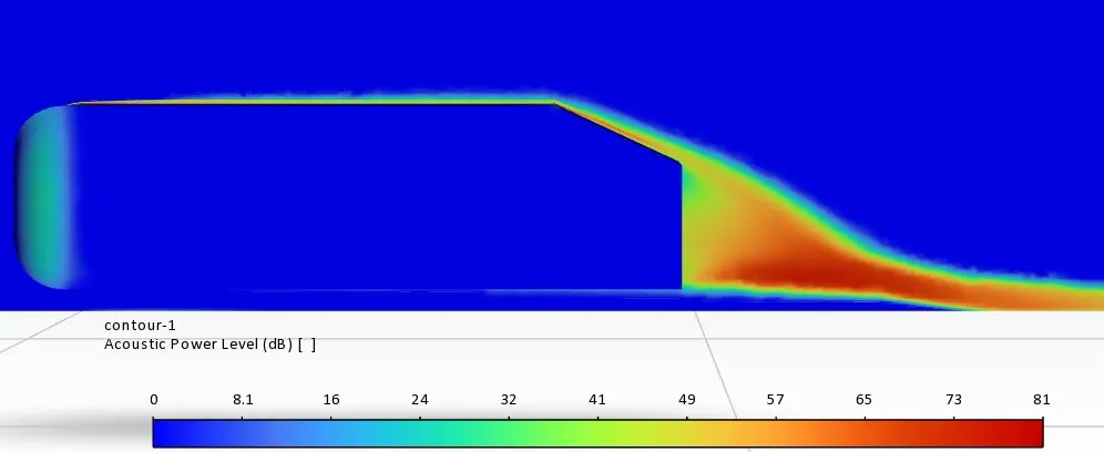
• Acoustic power level contour

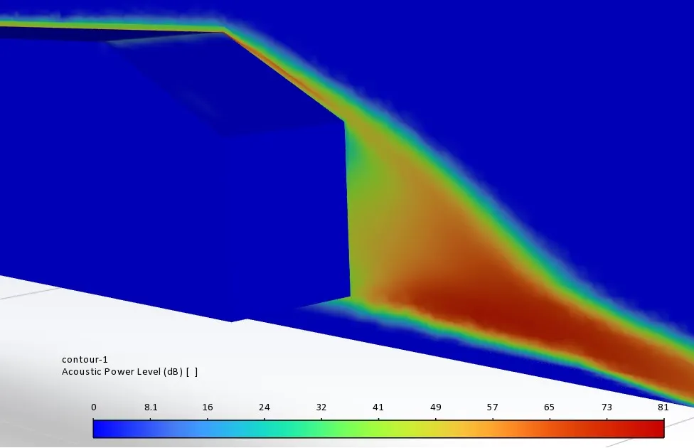
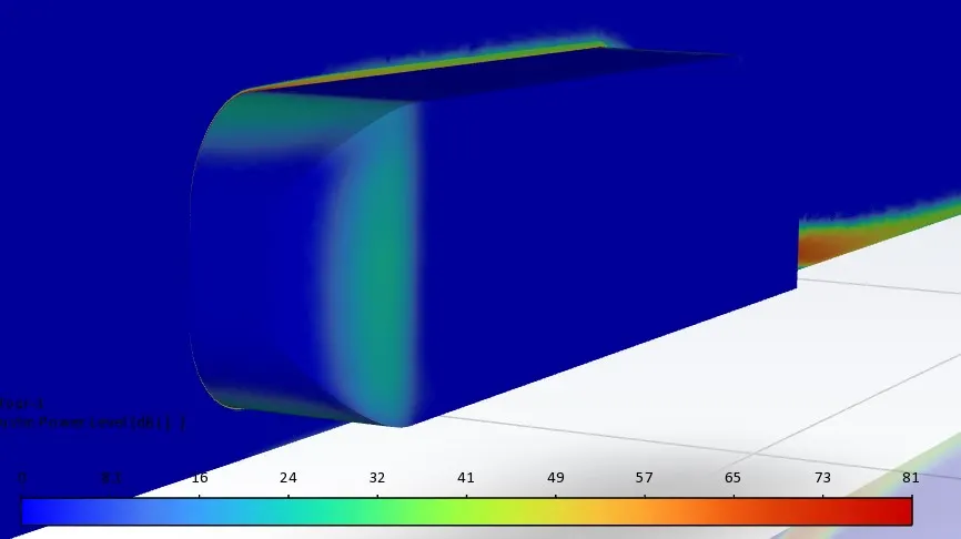
• Surface acoustic power level

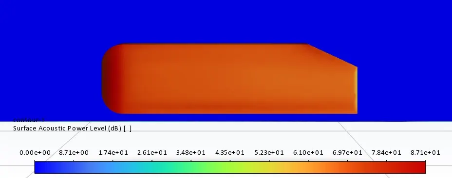
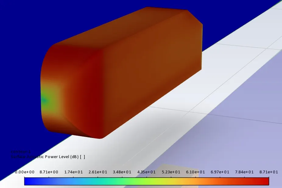
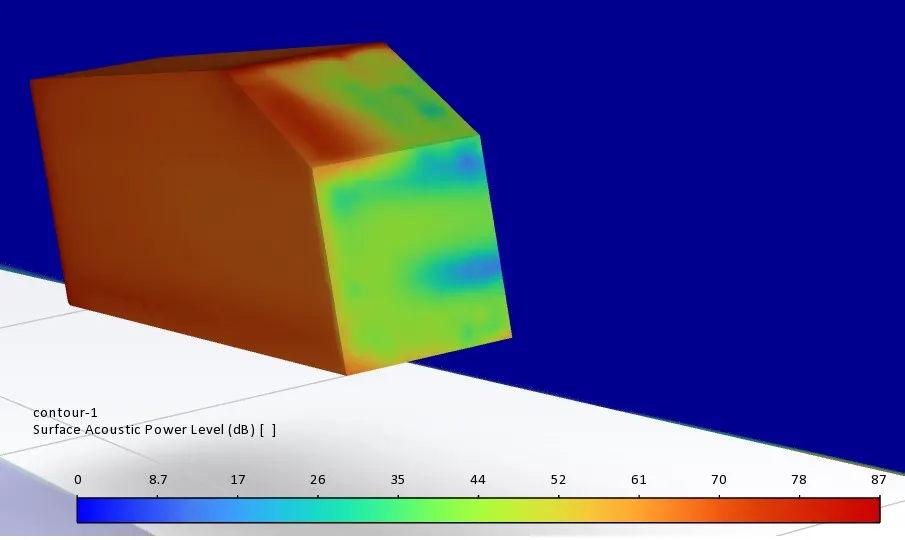
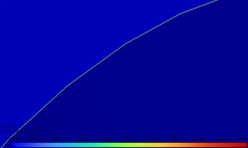
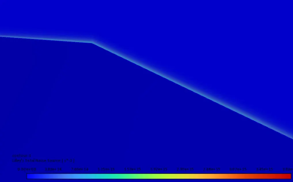
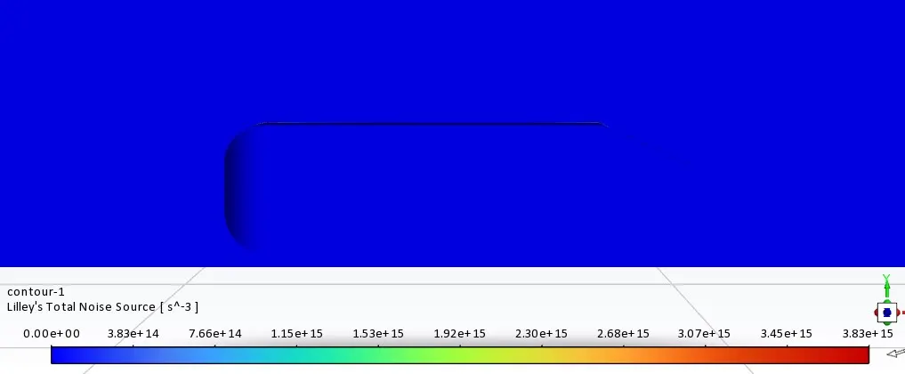
• Lily total noise source

Result:

Sr. No.	Parameters	Values
1	Coefficient of Drag	0.1472
2	Coefficient of Lift	0.155
3	Max. Velocity	47.23 m/s
4	Max. Static Pressure	578.37 Pa
	Min. Static Pressure	-1099.362 Pa
5	Max. Total Pressure	650.50 Pa
	Min. Total Pressure	-1089.97 Pa
6	Maximum Acoustic power level	81.057 db
7	Maximum Surface acoustic power level	87.09 db
8	Maximum Lily total noise source	3.83 x 10^15 s^-3

Conclusion:

• From the result obtained it is observed that the noise is generated in the low pressure regions of the ahmed body. Major contributors of noise are the curved frontal surface, inclined surface and wake region behind the ahmed body.
• By re engineering the design of the model noise generated can be minimised.