Week 7 - Simulation of a 1D Super-sonic nozzle flow simulation using Macormack Method

Description:
Here, we try to study quasi 1D supersonic nozzle. Inorder to do that we consider a convergent-divergent(CD) nozzle, which changes its crossection area along the x direction only. Further we assumw that air flows from a very large reservior so velocity is small, pressure and density of air are assumed to be atmospheric.

Now let us consider a small section on the CD nozzle along the x axis, since we are studying the changes in the primitive variables through 1D supersonic nozzle so we consider the any changes of the primitive variables along the y direction is same or we neglect we consider only the changes along the x direction.

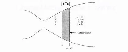
The flow velocity along the convergent section of the nozzle is subsonic(M<1) and at the throat it is sonic(M=1) and at the divergent section it is supersonic(M>1)
For quasi 1D steady state isentropic nozzle flow the qoverning continuity, momentum and energy equation using non dimensional variables are givenn below

A) Non-Conservation form:
1. continutiy equation :

`(delrho')/(delt')=-rho'*((delV')/(delx'))-rho'*V'*((del(lnA'))/(delx'))-V'*((delrho')/(delx'))`

2. Momentum equation :

`(delV')/(delt')=-V'*(delV')/(delx')-(1/gamma)*((delT')/(delx')+((T')/(rho')*(delrho')/(delx')))`

3. Energy equation :

`(delT')/(delt')=-V'*(delT')/(delx')-(gamma-1)*T'*((delV')/(delx')+V'*(del(lnA'))/(delx'))`

B) Conservation form:
1. continutiy equation :

`(delrho'*A')/(delt')+(delrho'*A'*V')/(delx')=0`

2. Momentum equation :

`(del(rho'*A'*V"))/(delt')+(del((rho'*A'*(V')^2)+(1/gamma)*rho'*A'))/(delx')=(1/gamma)*rho'*(delA')/(delx')`

3. Energy equation :

`(del(rho'*(e')/(gamma-1)+(gamma/2)*(V')^2)A')/(delt')+(del((rho'*(e')/(gamma-1)+(gamma/2)*(V')^2)*A'*V'+(rho'*A'*V')))/(delx')=0`

Main Program:
In the main program we providde the constant values of courant no. (for system stability ), gamma (for air it is 1.4), timestep values and the different values of node in the array. Then we call non conservative form and conservative form function with the required return variables, which we use to plot graph. Inorder to study the properties of flow along the CD nozzle we make use of Mackcormack technique

clear all
close all
clc

%mesh
node=[31,62,93];

C=.5;
%timetep iniialization
time=1400;

gamma=1.4;


    %non conservation form
    tic
    [x,n,throat_nc,mass_flow_nc,mass_flow_throat_nc,rho_throat_nc,t_throat_nc,pressure_throat_nc,mach_throat_nc,rho_nc,t_nc,pressure_nc,mach_nc,a_nc]=oneDsupersonic_NC(node(1),C,time,gamma);
    sim_time_nc=toc;

    %conservation form 
    tic
    [x,mass_flow_con,mass_flow_throat_con,rho_throat_con,t_throat_con,pressure_throat_con,mach_throat_con,rho_con,t_con,pressure_con,mach_con,a_con]=oneDsupersonic_con(node(1),C,time,gamma);
    sim_time_con=toc;


%plotting non conservation 
%timestep variation of primitive value at throat for non conservation form 
figure(1)
plot(linspace(1,time,time),rho_throat_nc,'m');
hold on
%temperature
plot(linspace(1,time,time),t_throat_nc,'c');
hold on
plot(linspace(1,time,time),pressure_throat_nc,'g');
hold on
plot(linspace(1,time,time),mach_throat_nc,'r');
hold on
xlabel('Timestep')
legend({'Density','Temperature','Pressure','Mach'});
grid minor;
title({'Timestep variation at throat area - Non Conservation Form';['Node =',num2str(n)]})

%flow rate distribution of primitive variables
figure(3)
%density
plot(x,rho_nc,'m','linewidth',1);
hold on
plot(x,t_nc,'c','linewidth',1);
hold on
plot(x,pressure_nc,'g','linewidth',1);
hold on
plot(x,mach_nc,'r','linewidth',1);
hold on
plot(x,a_nc,'k','linewidth',1.5);
hold on
xlabel('Domain Length')
legend({'Density','Temperature','Pressure','Mach Number','Area'});
grid minor;
title({'variation of flowrate distribution - Non Conservation Form';['Node =',num2str(n)]})

    
%plotting conservation 
%timestep variation of primitive value at throat for conservation form 
figure(5)
%density
plot(linspace(1,time,time),rho_throat_con,'m');
hold on
%temperature
plot(linspace(1,time,time),t_throat_con,'c');
hold on
%pressure
plot(linspace(1,time,time),pressure_throat_con,'g');
hold on
%mach number
plot(linspace(1,time,time),mach_throat_con,'r');
hold on
xlabel('Timestep')
legend({'Density','Temperature','Pressure','Mach'});
%axis([0 1400 0.6 .7]);
grid minor;
title({'Timestep variation at throat area - Conservation Form';['Node =',num2str(n)]})

%flow rate distribution of primitive variables
figure(6)
%density
plot(x,rho_con,'m','linewidth',1);
hold on
%tempertaure
plot(x,t_con,'c','linewidth',1);
hold on
%pressure
plot(x,pressure_con,'g','linewidth',1);
hold on
%Mach number
plot(x,mach_con,'r','linewidth',1);
hold on
%Nozzle area
plot(x,a_nc,'k','linewidth',1.5);
hold on
xlabel('Domain Length')
legend({'Density','Temperature','Pressure','Mach number','Nozzle area'});
grid minor;
title({'variation of flowrate distribution - Conservation Form';['Node =',num2str(n)]})

figure(7)
plot(x,mass_flow_nc,'b');
hold on
plot(x,mass_flow_con,'r');
hold on
xlabel('Length of Domain')
ylabel('Mass Flow Rate')
legend('Non Conserveration','Conservation');
title({'Normalized comparison of Conservation & Non-Conservation form ';['Node =',num2str(n)]})
grid on;

%grid dependency test
figure(8)
subplot(2,1,1)
plot(x,mass_flow_nc,'r');
hold on
xlabel('Length of Domain')
ylabel('Mass Flow Rate')
title({'Grid Dependency test for Non-Conservation Form at';['Node =',num2str(n)]})
grid on;

figure(9)
subplot(2,1,1)
plot(linspace(1,time,time),mass_flow_throat_nc,'r');
hold on
xlabel('Timestep')
ylabel('Mass Flow Rate')
title({'Grid Dependency test for Non-Conservation Form at';['Node =',num2str(n)]})
grid on;

figure(10)
subplot(2,1,1)
plot(x,mass_flow_con,'r');
hold on
xlabel('Length of Domain')
ylabel('Mass Flow Rate')
title({'Grid Dependency test for Conservation Form at';['Node =',num2str(n)]})
grid on;

figure(11)
subplot(2,1,1)
plot(linspace(1,time,time),mass_flow_throat_con,'r');
hold on
xlabel('Timestep')
ylabel('Mass Flow Rate')
title({'Grid Dependency test for Conservation Form at';['Node =',num2str(n)]})
grid on;

Sub Program1: (Non-Conservative form)

Initial condition:

• `rho=1-.3146*x` (Density)
• `T=1-.2314*x` (Temperature)
• `V=(0.1+1.09x)*sqrt(T)` (Velocity)
• `A=1+2.2*(x-1.5)^2` `0<=x<=3` (Area)

Macormack method:

1) Predictor step:(forward differencing)

`(deltarho)/(deltat)=-rho^n(i)*(V^n(i+1)-V^n(i))/(Deltax)-rho^n(i)*V(i)^n*((ln(A(i+1)-ln(A(i)))/(Deltax))-V^n(i)*((rho^n(i+1)-rho^n(i))/(Deltax))`

2) Solution update:

`rho(update)=rho(i)(Initial)+((deltarho)/(deltat))(Predictor)*dt`

3) Corrector step:(backward differencing) use updated rho value.

`(deltarho)/(deltat)=-rho^n(i)*(V^n(i)-V^n(i-1))/(Deltax)-rho^n(i)*V(i)^n*((ln(A(i)-ln(A(i-1)))/(Deltax))-V^n(i)*((rho^n(i)-rho^n(i-1))/(Deltax))`

4) Average step: Take the average value of the predictor and corrector step

`(deltarho)/(deltat)(avg)=0.5*(((deltarho)/(deltat))p+((deltarho)/(deltat))c)`

5) Final updation: for 2nd time step take first time step value and solve he following equation

`rho(2nd )=rho(1st)+((deltarho)/(deltat))(avg)*deltat`

Similarly, solve the momentum and energy governing equation for Non-Conservation form .

function    [x,n,throat_nc,mass_flow_nc,mass_flow_throat_nc,rho_throat_nc,t_throat_nc,pressure_throat_nc,mach_throat_nc,rho_nc,t_nc,pressure_nc,mach_nc,a_nc]=oneDsupersonic_NC(node,C,time,gamma)
n=node;
x=linspace(0,3,node);
dx=x(2)-x(1);
%Initial condition

    rho_nc=1-.3146*x;
    t_nc=1-.2314*x;
    v_nc=(.1+1.09*x).*t_nc.^.5;
    a_nc=1+2.2*(x-1.5).^2;
    throat_nc=find(a_nc==1 | a_nc<1.002,1);
%non conservation equation
%time loop
for l=1:time
    %saving the old value 
    rho_old=rho_nc;    %density
    t_old=t_nc;    %temperature
    v_old=v_nc;    %velocity
    a_old=a_nc;    %area

    dt=min(C*dx./(sqrt(t_nc)+v_nc));

 %predictor step
    for i=2:node-1
        dvdx(i)=(v_nc(i+1)-v_nc(i))/dx;
        dlogadx(i)=(log(a_nc(i+1))-log(a_nc(i)))/dx;
        drhodx(i)=(rho_nc(i+1)-rho_nc(i))/dx;
        dtdx(i)=(t_nc(i+1)-t_nc(i))/dx;
        
        drhodt_p(i)=-(rho_nc(i)*dvdx(i))-(rho_nc(i)*v_nc(i)*dlogadx(i))-(v_nc(i)*drhodx(i));
        dvdt_p(i)=-(v_nc(i)*dvdx(i))-(1/gamma)*(dtdx(i)+(t_nc(i)/rho_nc(i))*drhodx(i));
        dtdt_p(i)=-(v_nc(i)*dtdx(i))-(gamma-1)*t_nc(i)*(dvdx(i)+v_nc(i)*dlogadx(i));
        
        %predictor step upadte
        rho_nc(i)=rho_old(i)+(drhodt_p(i)*dt);
        t_nc(i)=t_old(i)+(dtdt_p(i)*dt);
        v_nc(i)=v_old(i)+(dvdt_p(i)*dt);
    end
    %corrector step
    for k=2:node-1
        dvdx(k)=(v_nc(k)-v_nc(k-1))/dx;
        dlogadx(k)=(log(a_nc(k))-log(a_nc(k-1)))/dx;
        drhodx(k)=(rho_nc(k)-rho_nc(k-1))/dx;
        dtdx(k)=(t_nc(k)-t_nc(k-1))/dx;
        
        drhodt_c(k)=-(rho_nc(k)*dvdx(k))-(rho_nc(k)*v_nc(k)*dlogadx(k))-(v_nc(k)*drhodx(k));
        dvdt_c(k)=-(v_nc(k)*dvdx(k))-(1/gamma)*(dtdx(k)+(t_nc(k)/rho_nc(k))*drhodx(k));
        dtdt_c(k)=-(v_nc(k)*dtdx(k))-(gamma-1)*t_nc(k)*(dvdx(k)+v_nc(k)*dlogadx(k));
    end
         %average step
        drhodt_avg=.5*(drhodt_p+drhodt_c);
        dvdt_avg=.5*(dvdt_p+dvdt_c);
        dtdt_avg=.5*(dtdt_p+dtdt_c);
    
    for i=2:node-1  
        %update
        rho_nc(i)=rho_old(i)+drhodt_avg(i)*dt;
        v_nc(i)=v_old(i)+dvdt_avg(i)*dt;
        t_nc(i)=t_old(i)+dtdt_avg(i)*dt;
    end
    
    %inlet and outlet boundary condition
    %inlet
    rho_nc(1)=1;
    t_nc(1)=1;
    v_nc(1)=2*v_nc(2)-v_nc(3);
    
    %outlet
    v_nc(node)=2*v_nc(node-1)-v_nc(node-2);
    rho_nc(node)=2*rho_nc(node-1)-rho_nc(node-2);
    t_nc(node)=2*t_nc(node-1)-t_nc(node-2);
    
    %defining mach no.,pressure,mass flow rate
    mass_flow_nc=rho_nc.*a_nc.*v_nc;
    pressure_nc=rho_nc.*t_nc;
    mach_nc=v_nc./sqrt(t_nc);
    
    %calculateing variables at throat
    rho_throat_nc(l)=rho_nc(throat_nc);
    v_throat_nc(l)=v_nc(throat_nc);
    t_throat_nc(l)=t_nc(throat_nc);
    mass_flow_throat_nc(l)=mass_flow_nc(throat_nc);
    pressure_throat_nc(l)=pressure_nc(throat_nc);
    mach_throat_nc(l)=mach_nc(throat_nc);
       
  
    %plotting
    %comparison of mass flow rate at different time step
    figure(4)
    if l==50
        mass_flow_nc_50=mass_flow_nc;
        plot(x,mass_flow_nc,'m','linewidth',1.25);
        hold on
    elseif l==100
        plot(x,mass_flow_nc,'c','linewidth',1.25);
        hold on
    elseif l==200
        plot(x,mass_flow_nc,'g','linewidth',1.25);
        hold on
    elseif l==400
        plot(x,mass_flow_nc,'y','linewidth',1.25);
        hold on
    elseif l==800
        plot(x,mass_flow_nc,'k','linewidth',1.25);
        hold on
    end
   
end
    %labelling
    title({'Mass flow rate at different timestep for Non-Conservation Form';['Node =',num2str(node)]})
    xlabel('Length of Domain')
    ylabel('Mass flow rate')
    legend({'50^t^h timestep','100^t^h timestep','200^t^h timestep','400^t^h timestep','800^t^h timestep'})
    %axis([0 3 0 2])
   
end

Output1:

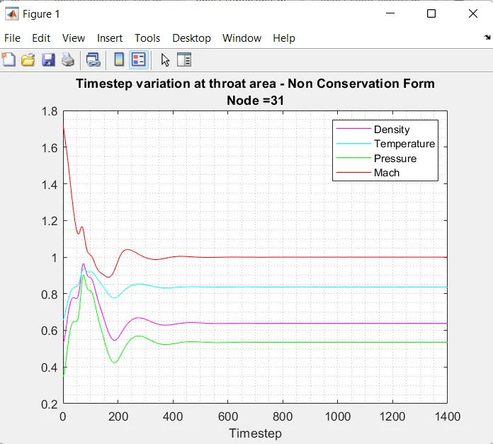
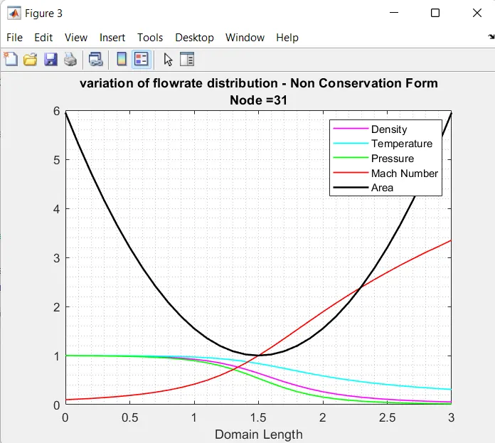
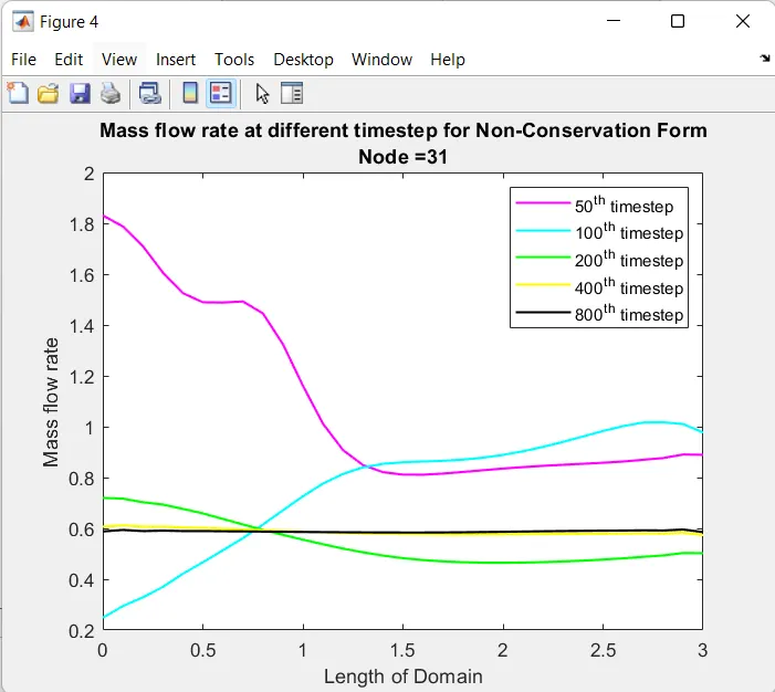
• Primitive values of the non conservation form when plotted for the 1400 timestep it is observed that solution starts to converge after 600th time step.
• When the primitive values of the non conservation form when plotted along the length of the nozzle it is observed that pressure, density and tempertaure starts to fall along the nozzle. whereas the mach no. starts to increase from subsonic region in converging section to sonic in throat and supersonic along the diverging section.
• When the mass flow rate is plotted along the length of the nozzle for different time step value it is observed that after 400th timestep the solution starts to converge.

Sub Program2: (Conservative form)

Initial condition :

• `A=1+2.2*(x-1.5)^2` `0<=x<=3`
• `rho' =1.0` `0<=x'<=0.5`

`T' = 1.0`

• `rho'=1-.366*(x'-0.5)` `.5<=x'<=1.5`

`T'=1-.167*(x'-0.5)`

• `rho' =.634-.3879*(x'-1.5)` `1.5<=x'<=3.5`

`T' =.833-.3507*(x'-1.5)`

• `V'=0.59/(rho '*A')`

Macormack method: Similar to Non conservation, solve the Conservation form of the momentum, continuity and energy governing equation. Also refer to code below for additional information.

function[x,mass_flow_con,mass_flow_throat_con,rho_throat_con,t_throat_con,pressure_throat_con,mach_throat_con,rho_con,t_con,pressure_con,mach_con,a_con]=oneDsupersonic_con(node,C,time,gamma)

x=linspace(0,3,node);
dx=x(2)-x(1);
%initial condition
for i=1:node
    if (x(i)>=0 && x(i)<=.5)
        rho_con(i)=1;
        t_con(i)=1;
    elseif (x(i)>.5 && x(i)<=1.5)
        rho_con(i)=1-.366*(x(i)-.5);
        t_con(i)=1-.167*(x(i)-0.5);
    elseif (x(i)>1.5 && x(i)<=3.5)
        rho_con(i)=.634-.3879*(x(i)-1.5);
        t_con(i)=.833-.3507*(x(i)-1.5);
    end


    %initial velocity and pressure profile
    a_con(i)=1+(2.2*(x(i)-1.5)^2);
    throat=find(a_con==1 | a_con<1.002,1);
    v_con(i)=.59/(rho_con(i)*a_con(i));
    pressure_con(i)=rho_con(i)*t_con(i);

    %initial solution vector
    u1_con(i)=rho_con(i)*a_con(i);
    u2_con(i)=rho_con(i)*a_con(i)*v_con(i);
    u3_con(i)=rho_con(i)*((t_con(i)/(gamma-1))+(0.5*gamma*v_con(i)^2))*a_con(i);
end

%time loop
for l=1:time
     %saving the old value 
    rho_old=rho_con;    %density
    t_old=t_con;    %temperature
    v_old=v_con;    %velocity
    u1_old_con=u1_con;
    u2_old_con=u2_con;
    u3_old_con=u3_con;

    dt=min(C*dx./(sqrt(t_con)+v_con));
    
    for i=1:node
    %initialization of flux variable
        f1_con_p(i)=u2_con(i);
        f2_con_p(i)=((u2_con(i)^2)/u1_con(i))+(((gamma-1)/gamma)*(u3_con(i)-((gamma*(u2_con(i)^2))/(2*u1_con(i)))));
        f3_con_p(i)=((gamma*u2_con(i)*u3_con(i))/u1_con(i))-((gamma*(gamma-1)*(u2_con(i)^3))/(2*(u1_con(i)^2)));
    end
    
    %predictor step
    for j=2:node-1
        j2_con_p(j)=(1/gamma)*rho_con(j)*t_con(j)*((a_con(j+1)-a_con(j))/dx);

        %predictor flux
        df1dx_con_p(j)=(f1_con_p(j+1)-f1_con_p(j))/dx;
        df2dx_con_p(j)=(f2_con_p(j+1)-f2_con_p(j))/dx;
        df3dx_con_p(j)=(f3_con_p(j+1)-f3_con_p(j))/dx;
        
        du1dt_con_p(j)=-df1dx_con_p(j);
        du2dt_con_p(j)=-df2dx_con_p(j)+j2_con_p(j);
        du3dt_con_p(j)=-df3dx_con_p(j);
        
        %update predicted value
        u1_con(j)=u1_old_con(j)+(du1dt_con_p(j)*dt);
        u2_con(j)=u2_old_con(j)+(du2dt_con_p(j)*dt);
        u3_con(j)=u3_old_con(j)+(du3dt_con_p(j)*dt);
    end
    for i=1:node
        %primitive value
        rho_con(i)=u1_con(i)/a_con(i);
        t_con(i)=(gamma-1)*((u3_con(i)/u1_con(i))-(.5*gamma*v_con(i)^2));
        v_con(i)=u2_con(i)/u1_con(i);
        pressure_con(i)=rho_con(i)*t_con(i);
    end
    
    %corrector step
    for i=1:node
    %initialization of flux variable
        f1_con_c(i)=u2_con(i);
        f2_con_c(i)=((u2_con(i)^2)/u1_con(i))+(((gamma-1)/gamma)*(u3_con(i)-((gamma*(u2_con(i)^2))/(2*u1_con(i)))));
        f3_con_c(i)=((gamma*u2_con(i)*u3_con(i))/u1_con(i))-((gamma*(gamma-1)*(u2_con(i)^3))/(2*(u1_con(i)^2)));
    end
    for j=2:node-1
        j2_con_c(j)=(1/gamma)*pressure_con(j)*((a_con(j)-a_con(j-1))/dx);

        df1dx_con_c(j)=((f1_con_c(j)-f1_con_c(j-1))/dx);
        df2dx_con_c(j)=(f2_con_c(j)-f2_con_c(j-1))/dx;
        df3dx_con_c(j)=(f3_con_c(j)-f3_con_c(j-1))/dx;
        
        du1dt_con_c(j)=-df1dx_con_c(j);
        du2dt_con_c(j)=-df2dx_con_c(j)+j2_con_c(j);
        du3dt_con_c(j)=-df3dx_con_c(j);     
    end
    %average
    for i=2:node-1
        du1dt_con_avg(i)=(du1dt_con_p(i)+du1dt_con_c(i))/2;
        du2dt_con_avg(i)=(du2dt_con_p(i)+du2dt_con_c(i))/2;
        du3dt_con_avg(i)=(du3dt_con_p(i)+du3dt_con_c(i))/2;
    
        %final solution
        u1_con(i)=u1_old_con(i)+(du1dt_con_avg(i)*dt);
        u2_con(i)=u2_old_con(i)+(du2dt_con_avg(i)*dt);
        u3_con(i)=u3_old_con(i)+(du3dt_con_avg(i)*dt);   
    end
    %boundary condition
    %subsonic inflow
    u1_con(1)=rho_con(1)*a_con(1);
    u2_con(1)=(2*u2_con(2))-u2_con(3);
    u3_con(1)=u1_con(1)*((t_con(1)/(gamma-1))+(gamma*.5*v_con(1)^2));
    %supersonic outflow
    u1_con(node)=(2*u1_con(node-1))-u1_con(node-2);
    u2_con(node)=(2*u2_con(node-1))-u2_con(node-2);
    u3_con(node)=(2*u3_con(node-1))-u3_con(node-2);
    
    for i=1:node
        %primitive value
        rho_con(i)=u1_con(i)/a_con(i);
        v_con(i)=u2_con(i)/u1_con(i);
        t_con(i)=(gamma-1)*((u3_con(i)/u1_con(i))-(.5*gamma*(v_con(i)^2)));
        pressure_con(i)=rho_con(i)*t_con(i);
        mach_con(i)=(v_con(i)/(sqrt(t_con(i))));
        mass_flow_con(i)=rho_con(i)*a_con(i)*v_con(i);
    end
   
    %calculateing variables at throat
    rho_throat_con(l)=rho_con(throat);
    v_throat_con(l)=v_con(throat);
    t_throat_con(l)=t_con(throat);
    mass_flow_throat_con(l)=mass_flow_con(throat);
    pressure_throat_con(l)=pressure_con(throat);
    mach_throat_con(l)=mach_con(throat);
        

 if node==31   
    %plotting
    %comparison of mass flow rate at different time step
    figure(2)
    if l==50
        plot(x,mass_flow_con,'m','linewidth',1.25);
        hold on
    elseif l==100
        plot(x,mass_flow_con,'c','linewidth',1.25);
        hold on
    elseif l==200
        plot(x,mass_flow_con,'g','linewidth',1.25);
        hold on
    elseif l==400
        plot(x,mass_flow_con,'y','linewidth',1.25);
        hold on
    elseif l==800
        plot(x,mass_flow_con,'k','linewidth',1.25);
        hold on
    end
 end
end
    %labelling
    title({'Mass flow rate at different timestep for Conservation Form';['Node =',num2str(node)]})
    xlabel('Length of Domain')
    ylabel('Mass flow rate')
    legend({'50^t^h timestep','100^t^h timestep','200^t^h timestep','400^t^h timestep','800^t^h timestep'})
    axis([0 3 0.4 1])
    end
    

Output2:

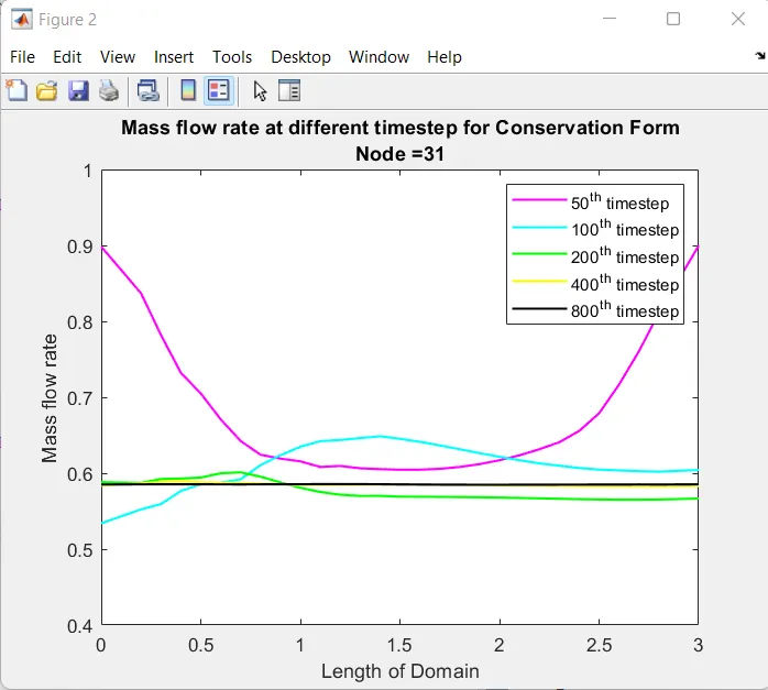
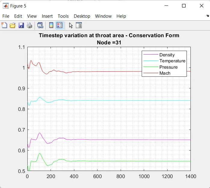
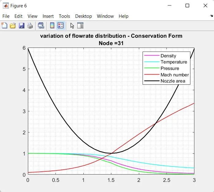
• When the mass flow rate is plotted along the length of the nozzle for different time step value it is observed that after 100th timestep the solution starts to converge and stablizies in the 800th timestep.
• Primitive values of the conservation form when plotted for the 1400 timestep it is observed that solution starts to converge after 600th time step.
• When the primitive values of the conservation form is plotted along the length of the nozzle it is observed that pressure, density and tempertaure starts to fall along the nozzle. whereas the mach no. starts to increase from subsonic region in converging section to sonic in throat and supersonic along the diverging section. Nozzle outline area is plotted in black to get the idea of region in nozzle along with the primitive values plot.

Comparision of conservation & non-conservation form :

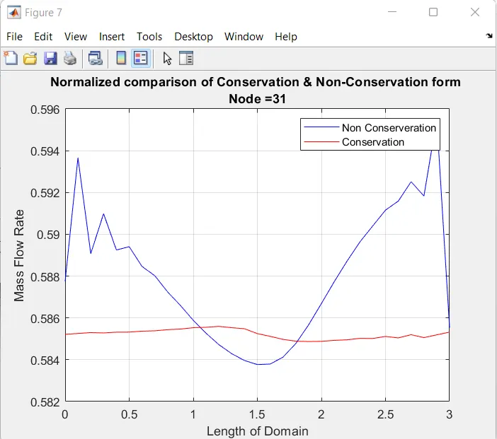
• The difference between both the form is very small. The mass flow rate in the Conservation form is converges faster than the Non-Conservation form.
• We can conclude that the final solution does not change much when using Conservation and Non-Conservation form.

Grid Dependency Test: Inorder to check whether the solution depends on number of grid points or not grid dependency test is carried out. if yes, then the solution cannot be taken into consideration.

A) Non-Conservation Form

1)Massflow rate Vs Domain length

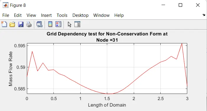
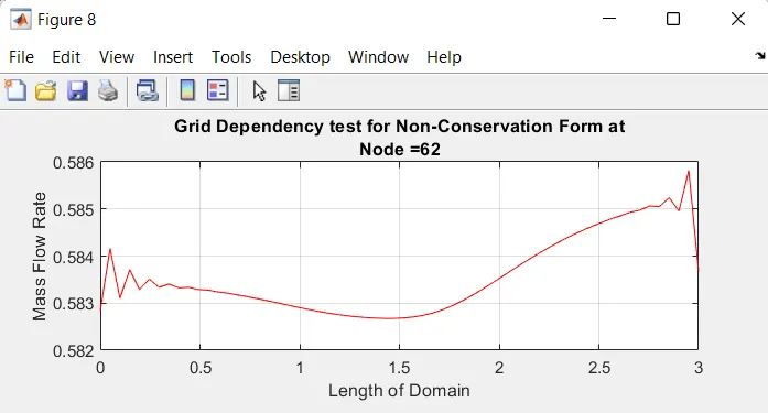
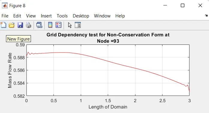
• when mass flow rate is plotted along the length of the nozzle for different nodal points the solution does not differ much and still lie within the range of acceptance

2)Massflow rate (Throat) Vs Timestep

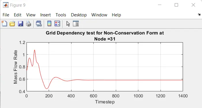
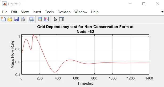
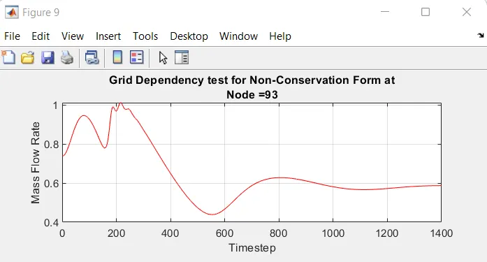
• When the mass flow rate at the throat is plotted against 1400 time step for different nodal points, it is seen that as the nodal points are increased the converges of solution takes place with increased no. of time step.

B) Conservation Form

1)Massflow rate Vs Domain length

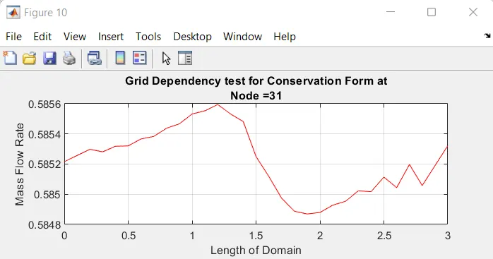
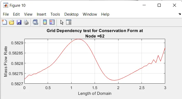
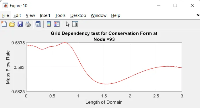
• when mass flow rate is plotted along the length of the nozzle for different nodal points the solution does not differ much and still lie within the range of acceptance
• It is also seen that as the nodal points are increased the peaks and valleys in the graph smoothens out.

2)Massflow rate (Throat) Vs Timestep

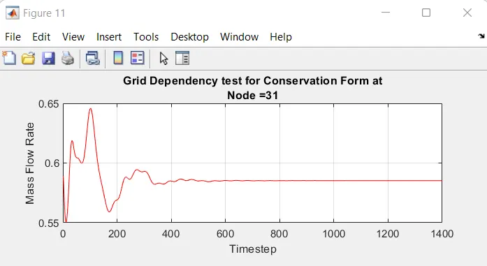
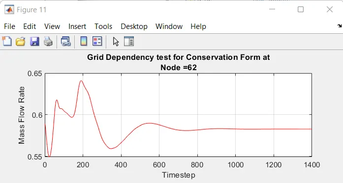
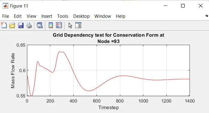
• When the mass flow rate at the throat is plotted against 1400 time step for different nodal points, it is seen that as the nodal points are increased the convergance of solution takes place with increased no. of time step.
• The curve also observed to be smoother as the nodal points are increased.

Result:

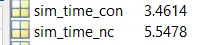
• Coding the Non conservation form is much more simpler then the onservation form.
• Eventhough the conservation and non conservation form deliver similar result it is observed that solution converges faster for the conservation form.
• If given a choice then conservation form should be picked for the solution.