Week 3.5 - Deriving 4th order approximation of a 2nd order derivative using Taylor Table method

Explanation:

In order to solve the 2^nd order differential equation using Taylor table method we need to find no. of node necessary for symmetric and asymmetric stencil.

• For Symmetric stencil: ( central scheme )

no. of nodes = (order of accuracy) + (order of derivative) – 1

i.e. no. of nodes = 4 + 2 – 1 = 5

• For Asymmetric stencil: ( Skewed scheme )

no. of nodes = (order of accuracy) + (order of derivative)

i.e. no. of nodes = 4 + 2 = 6

Central scheme : ( using Taylor table )

Taylor series :

f(x) = f(x) + x*f(x)/1 + x^2*f’(x)/2! + x^3*f’’(x)/3! + …… + x^n*fⁿ(x)/n!

	f( i )	∆x*f’( i )	∆x*f’’( i )	∆x*f’’’( i )	∆x*f’v( i )
a*f( i - 2 )	a	-2a	4a/2	-8a/6	16a/24
b*f( i – 1 )	b	-b	b/2	-b/6	b/24
c*f( i )	c	0	0	0	0
d*f( i + 1 )	d	d	d/2	d/6	d/24
e*f( i + 2 )	e	2e	4e/2	8e/6	16e/24
	0	0	1	0	0

Solving the equation

a + b + c + d + e = 0

-2a – b + d + 2e = 0

4a/2 + b/2 + d/2 + 4e/2 = 1

-8a/6 - b/6 + d/6 + 8e/6 = 0

16a/24 + b/24 + d/24 + 16e/24 = 0

Using the value of a, b, c, d, e solve the below equation

∆²u = [a*f( i – 2 ) + b*f( i – 1 ) + c*f( i ) + d*f( i + 1 ) + e*f( i + 2 )] / ( dx )^2

Right skewed scheme : ( using Taylor table )

	f( i )	∆x*f’( i )	∆x*f’’( i )	∆x*f’’’( i )	∆x*f’v( i )	∆x*fv( i )
a*f( i )	a	0	0	0	0	0
b*f( i + 1 )	b	b	b/2	b/6	b/24	b/120
c*f( i + 2 )	c	2c	2c	8c/6	16c/24	32c/120
d*f( i + 3 )	d	3d	9d/2	27d/6	81d/24	243d/120
e*f( i + 4 )	e	4e	16e/2	64e/6	256e/24	1024e/120
f*f( i + 5 )	f	5f	25f/2	125f/6	625f/24	3125f/120
	0	0	1	0	0	0

Solve the equation

a + b + c + d + e + f = 0

b + 2c + 3d + 4e + 5f = 0

b/2 + 2c + 9d/2 + 16e/2 + 25f/2 = 1

b/6 + 8c/6 + 27d/6 + 64e/6 + 125f/6 = 0

b/24 + 16c/24 + 81d/24 + 256e/24 + 625f/24 = 0

b/120 + 32c/120 + 243d/120 + 1024e/120 + 3125f/120 = 0

Using the value of a, b, c, d, e, f solve the below equation

∆²u = [a*f( i ) + b*f( i + 1 ) + c*f( I + 2 ) + d*f( i + 3 ) + e*f( i + 4 ) + f*f( i + 5 )] / ( dx )^2

Left skewed scheme :

Similarly follow the steps of right skewed scheme.

PROGRAM CODE :

clear all
close all
clc

%central differencing
A=[1 1 1 1 1; -2 -1 0 1 2; 2 1/2 0 1/2 2; -8/6 -1/6 0 1/6 8/6; 16/24 1/24 0 1/24 16/24]
M=[0;0;1;0;0]

P=A\M

%right side skewed differencing
B=[1 1 1 1 1 1; 0 1 2 3 4 5; 0 1/2 2 9/2 8 25/2; 0 1/6 8/6 27/6 64/6 125/6; 
    0 1/24 16/24 81/24 256/24 625/24; 0 1/120 32/120 243/120 1024/120 3125/120]
N=[0;0;1;0;0;0]
Y=B\N

%left side skewed differecing
C=[1 1 1 1 1 1; -5 -4 -3 -2 -1 0; 25/2 8 9/2 2 1/2 0; -125/6 -64/6 -27/6 -8/6 -1/6 0;
       625/24 256/24 81/24 16/24 1/24 0; -3125/120 -1024/120 -243/120 -32/120 -1/120 0]
Z=C\N

x=pi/3;
dx=linspace(pi/20, pi/200,20);

%exact 2nd order derivative of analytic function e^x*cos(x)
exact_derivative=(-2)*exp(x)*sin(x);
for i=1:length(dx)
    central_diff_error(i)=central_diff(exact_derivative,P,x,dx(i));
    
    
   right_skewed_diff_error(i)=right_skewed_diff(exact_derivative,Y,x,dx(i));
    
    
    left_skewed_diff_error(i)=left_skewed_diff(exact_derivative,Z,x,dx(i));
end

%plotting result
figure(1)
loglog(dx,central_diff_error,'linewidth',3)
hold on
loglog(dx,right_skewed_diff_error,'r','linewidth',3)
hold on 
loglog(dx,left_skewed_diff_error,'g','linewidth',3)
xlabel('Range of dx')
ylabel('Absolute Error')
legend('central_diff_error','right_skewed_diff_error','left_skewed_diff_error')

Function for Central scheme :

function error=central_diff(exact_derivative,P,x,dx)
%central_diff=(a*f(x-2dx)+b*f(x-dx)+c*f(x)+d*f(x+dx)+e*f(x+2dx))/dx^2
%f(x)=exp(x)*cos(x)
f_1=exp(x-(2*dx))*cos(x-(2*dx));
f_2=exp(x-dx)*cos(x-dx);
f_3=exp(x)*cos(x);
f_5=exp(x+(2*dx))*cos(x+(2*dx));
f_4=exp(x+dx)*cos(x+dx);
central_diff=((P(1)*f_1)+(P(2)*f_2)+(P(3)*f_3)+(P(4)*f_4)+(P(5)*f_5))/(dx^2);
error= abs(exact_derivative-central_diff);
end

now, we calculate the absolute error by subtracting exact derivative value with central difference value

Function for Right scheme :

function error=right_skewed_diff(exact_derivative,Y,x,dx)
%right_skewed_diff=(A*f(x)+B*f(x+dx)+C*f(x+2dx)+D*f(x+3dx)+E*f(x+4dx))+F*f(x+5dx)/dx^2
%f(x)=exp(x)*cos(x)
f_1=exp(x)*cos(x);
f_2=exp(x+dx)*cos(x+dx);
f_3=exp(x+(2*dx))*cos(x+(2*dx));
f_4=exp(x+(3*dx))*cos(x+(3*dx));
f_5=exp(x+(4*dx))*cos(x+(4*dx));
f_6=exp(x+(5*dx))*cos(x+(5*dx));
right_skewed_diff=((Y(1)*f_1)+(Y(2)*f_2)+(Y(3)*f_3)+(Y(4)*f_4)+(Y(5)*f_5)+(Y(6)*f_6))/(dx^2);
error=abs(exact_derivative-right_skewed_diff)
end

similar to central scheme calculate the absolute error

Function for Left scheme :

function error=left_skewed_diff(exact_derivative,Z,x,dx)
%left_skewed_diff=(A*f(x)+B*f(x-dx)+C*f(x-2dx)+D*f(x-3dx)+E*f(x-4dx))+F*f(x-5dx)/dx^2
%f(x)=exp(x)*cos(x)
f_6=exp(x)*cos(x);
f_5=exp(x-dx)*cos(x-dx);
f_4=exp(x-(2*dx))*cos(x-(2*dx));
f_3=exp(x-(3*dx))*cos(x-(3*dx));
f_2=exp(x-(4*dx))*cos(x-(4*dx));
f_1=exp(x-(5*dx))*cos(x-(5*dx));
left_skewed_diff=((Z(1)*f_1)+(Z(2)*f_2)+(Z(3)*f_3)+(Z(4)*f_4)+(Z(5)*f_5)+(Z(6)*f_6))/(dx^2);
error=abs(exact_derivative-left_skewed_diff)
end

similar to central scheme calculate the absolute error

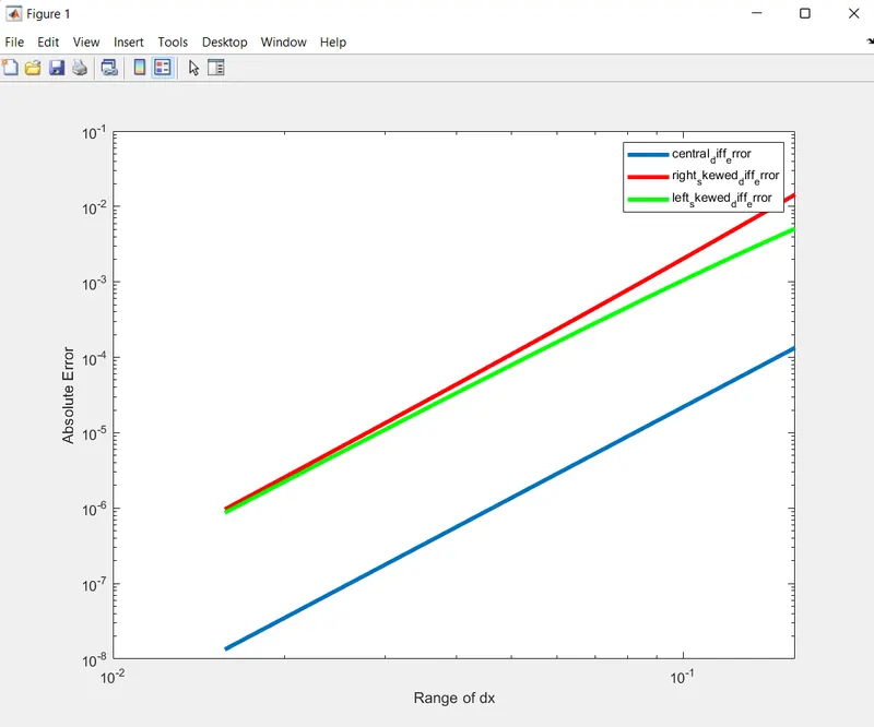
RESULT :

• By solving the program we get to see the result through graph
• From observtaion it seems that truncation error obtained from central scheme is less than the skewed scheme
• Right and Left scheme truncation error obtained are similar but larger then central scheme.

Graph :

Why skewed scheme is better than Central scheme ?

• Eventhough central scheme yields less truncation error than skewed scheme, it cannot be used in various boundary problems.
• In order to solve central scheme it require data from right and left side of the stencil, which becomes difficult in certain problems so it is better to solve the problem using skewed scheme.