Week 5.1 - Mid term project - Solving the steady and unsteady 2D heat conduction problem
Explanation:
2D conduction equation is given by,
`(delT)/(delt)=alpha*((del^2T)/(delx^2)+(del^2T)/(dely^2))`
so, by using the given values in the question the main program code is created.
Main Program:
clear all
close all
clc

%input
nx=30;
ny=nx;
x=linspace(0,1,nx);
dx=x(2)-x(1);
y=linspace(0,1,ny);
dy=y(2)-y(1);

%avg of BC on corner node
t=302*ones(nx,ny);
t(1,1)=500;
t(1,nx)=700;
t(ny,1)=650;
t(nx,ny)=850;

%input BC
t(1,2:nx-1)=600;
t(nx,2:ny-1)=900;
t(2:nx-1,1)=400;
t(2:nx-1,ny)=800;


told=t;
iterative_solver=3;
o_mega=1.2;
error=9e9;
tol=1e-4;


%steady state iterative function
figure(1)
[t1]=twoD_steady(iterative_solver,nx,ny,t,told,dx,dy,x,y,o_mega,error,tol);

%transient state implict iterative function
figure(2)
[t2]=twoD_cond_implict(iterative_solver,nx,ny,t,told,dx,dy,x,y,o_mega,error,tol);

%transient state explicit function
figure(3)
[t3]=twoD_cond_explict(nx,ny,t,told,dx,dy,x,y);
- The main program for the ode is created by keeping in mind that the whole transient(implict) and steady state solution be brought ,so that the iteration of, for example jacobi for transient (implict) and steady state and transient (explict) be called in a single call.
- The gride size for the x & y coordinate by defining the node size 30 for x & y coordinate.
- From the question boundary condition are defined and the corner node are taken the average of the two adjacent side condition.
- In the main program the type of iteration be called is given a initial value i.e. 1=Jacobi, 2=gauss seidal, 3=SOR.
- The function for transient (implict and explicit) and steady state is called by necessary input terms.
A) Steady state
- Discreatization of steady state 2D conduction equation is given by,
`(del^2T)/(delx^2)+(del^2T)/(dely^2)=0`
by using 2nd order central discreatization we get,
`(del^2T)/(del^2x)=(T(i-1)-2T(i)+T(i+1))/(Deltax^2)`
`(del^2T)/(del^2y)=(T(i-1)-2T(i)+T(i+1))/(Deltay^2)`
`Rightarrow T(i,j)=(1/k)*(T(i-1,j)+T(i+1,j))/(Deltax^2)+(1/k)*(T(i,j-1)+T(i,j+1))/(Deltay^2`
`k=2*(Deltax^2+Deltay^2)/(Deltax^2*Deltay^2)`
Sub_Program_1:
function [t1]=twoD_steady(iterative_solver,nx,ny,t,told,dx,dy,x,y,o_mega,error,tol)

%function req value;

if iterative_solver==1
    tic
    iter=1;
    while(error>tol)
        for i=2:nx-1
            for j=2:ny-1
               t(i,j)=(told(i-1,j)+told(i+1,j)+told(i,j-1)+told(i,j+1))*.25;
            end
        end
            error=max(max(abs(told-t)));
            told=t;
            iter=iter+1;
    end
    t1=toc;

elseif iterative_solver==2
    tic
    iter=1;
    while(error>tol)
        for i=2:nx-1
            for j=2:ny-1
               t(i,j)=(t(i-1,j)+told(i+1,j)+ t(i,j-1)+told(i,j+1))*.25;
            end
        end
            error=max(max(abs(told-t)));
            told=t;
            iter=iter+1;
    end
    t1=toc;

    elseif iterative_solver==3
        tic
    iter=1;
    while(error>tol)
        for i=2:nx-1
            for j=2:ny-1
                t(i,j)=(t(i-1,j)+told(i+1,j)+ t(i,j-1)+told(i,j+1))*.25;
                t(i,j)=(told(i,j)*(1-o_mega))+(o_mega*t(i,j));
            end
        end
            error=max(max(abs(told-t)));
            told=t;
            iter=iter+1;
    end
    t1=toc;

end

%plot
[c,h]=contourf(x,y,t);
clabel(c,h)
colorbar
colormap(turbo)
ax=gca;
ax.YDir='reverse';
xlabel('X-axis')
ylabel('Y-axis')
title({'Steady State Temperature Profile';['Iteration Method =',num2str(iterative_solver)];['No. of iterations=',num2str(iter)];['Simulation time=',num2str(t1),'s']})
grid on
- The steady state function for the given problem is created.
- The error from the iteration need to be less than 1e-4 so intitially the error is given 9e9 so that iteration be carried out within the while loop.
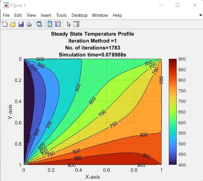
- For the iterative_solver value of 1 jacobian iteration be solved and there simulation time and total no. of iteration is also noted.
Result_1:
- Jacobi method
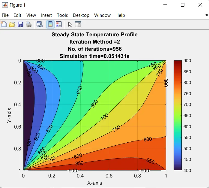
B. Gauss seidal method
C. Successive over relaxation (SOR) method
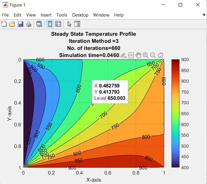
- From the result of the steadystate analysis it is clear that the SOR method converges faster with less no. of iteration
- Jacobi method converges slowly with large no. of iteration.
B) Transisent state (Implict method):
2D conduction equation for transisent state implicit equation is given by,
`T^(n+1)(i,j)=term*((k1*(T(i-1,j)+T(i+1,j)))+(k2*(T(i,j-1)+t(i,j+1)))+T^n(i,j)`
`term=(1+(2*k1)+(2*k2))^-1`
`k1=(alpha*(DeltaT)/(Deltax^2))`
`k2=(alpha*(DeltaT)/(Deltay^2))`
Sub_Program_2:
function[t2]=twoD_cond_implict(iterative_solver,nx,ny,t,told,dx,dy,x,y,o_mega,error,tol)

dt=3;
alpha=1.75e-2; %thermal diffusivity
k1=alpha*dt/dx^2;
k2=alpha*dt/dy^2;
term=(1+2*k1+2*k2)^-1;
t_prev=t;
time=200;
nt=time/dt;
cfl=alpha*dt*((1/dx^2)+(1/dy^2));

%jacobi method
if iterative_solver==1
    tic
    iter=1;
    for a=1:nt
      while(error>tol)
        for i=2:nx-1
            for j=2:ny-1
                h=k1*(told(i-1,j)+told(i+1,j));
                v=k2*(told(i,j-1)+told(i,j+1));
                t(i,j)=(t_prev(i,j)+h+v)*term;
            end
        end
            error=max(max(abs(told-t)));
            told=t;
            iter=iter+1;
    end
    t_prev=t;
    end
    t2=toc;


%gauss seidal method
elseif iterative_solver==2
    tic
    iter=1;
    for a=1:nt
      while(error>tol)
        for i=2:nx-1
            for j=2:ny-1
                h=k1*(t(i-1,j)+told(i+1,j));
                v=k2*(t(i,j-1)+told(i,j+1));
                t(i,j)=(t_prev(i,j)+h+v)*term;
            end
        end
            error=max(max(abs(told-t)));
            told=t;
            iter=iter+1;
    end
    t_prev=t;
    end
    t2=toc;

    %SOR method
    elseif iterative_solver==3
    tic
    iter=1;
    for a=1:nt
      while(error>tol)
        for i=2:nx-1
            for j=2:ny-1
                 h=k1*(t(i-1,j)+told(i+1,j));
                v=k2*(t(i,j-1)+told(i,j+1));
                t(i,j)=(t_prev(i,j)+h+v)*term;
                t(i,j)=told(i,j)*(1-o_mega)+o_mega*t(i,j);
            end
        end
            error=max(max(abs(told-t)));
            told=t;
            iter=iter+1;
    end
    t_prev=t;
    end
    t2=toc;

end
%plot
[c,h]=contourf(x,y,t);
clabel(c,h)
colorbar
colormap(turbo)
ax=gca;
ax.YDir='reverse';
xlabel('X-axis')
ylabel('Y-axis')
title({'Transient State Implict Temperature Profile';['Iteration Method =',num2str(iterative_solver)];['No. of iterations=',num2str(iter),'     Time=',num2str(time)];['CFL=',num2str(cfl),'     Error=',num2str(error)];['Simulation time=',num2str(t2),'s']})
grid on
Result_2:
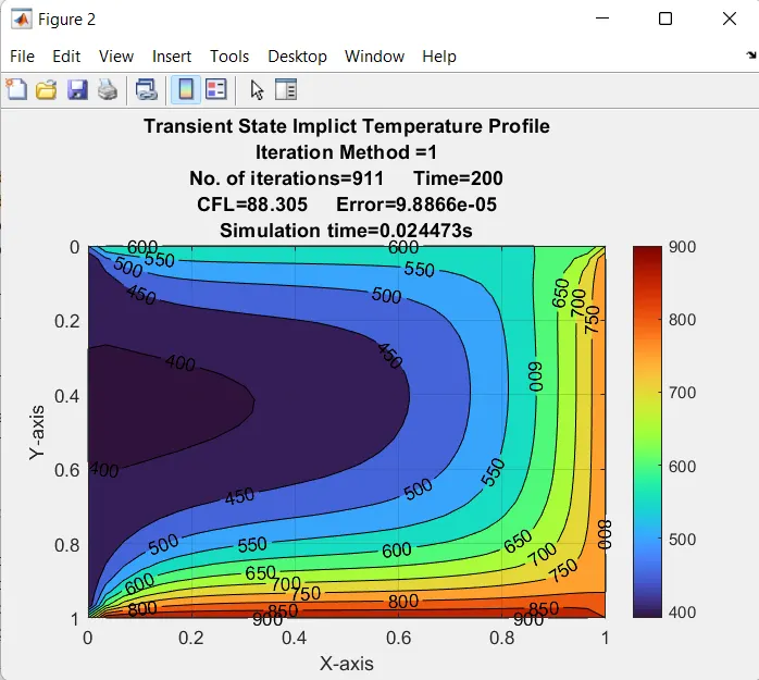
- Jacobi method
B. Gauss seidal method
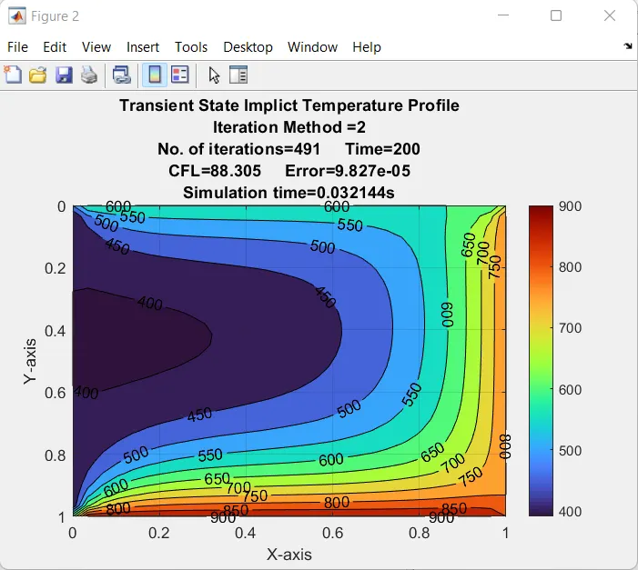
c. SOR method
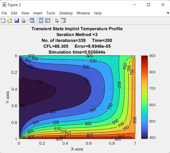
- From the results of the implict solution as well the SOR method coverges faster with less no. of iteration.
- Jacobi method completes the problem with large no. of iteration.
C) Transisent state (Explict method):
2D conduction equation for transisent state explicit method is given by,
`T^(n+1)(i,j)=T^n(i,j)+(k1*((T(i-1,j)-2T(i,j)+T(i+1,j))^n)+(k2*((T(i,j-1)-2T(i,j)+T(i,j+1))^n))`
`k1=alpha*(DeltaT)/(Deltax^2)`
`k2=alpha*(DeltaT)/(Deltay^2)`
Sub_Program_3:
function[t3]=twoD_cond_explict(nx,ny,t,told,dx,dy,x,y)
dt=.01;
alpha=1.75e-2; %thermal diffusivity
k1=(alpha*dt)/(dx^2);
k2=(alpha*dt)/(dy^2);
time=3;
nt=time/dt;
cfl=alpha*(dt/(dx^2));

%jacobi method
    tic
    iter=1;
    for a=1:nt
        for i=2:nx-1
            for j=2:ny-1
                h=k1*(told(i-1,j)-(2*told(i,j))+told(i+1,j));
                v=k2*(told(i,j-1)-(2*told(i,j))+told(i,j+1));
                t(i,j)=told(i,j)+h+v;
            end
        end
            error=max(max(abs(told-t)));
            told=t;
            iter=iter+1;
    end
    t3=toc;

%plot
[c,h]=contourf(x,y,t);
clabel(c,h)
colorbar
colormap(turbo)
ax=gca;
ax.YDir='reverse';
xlabel('X-axis')
ylabel('Y-axis')
title({'Transient State Explict Temperature Profile';['No. of iterations=',num2str(iter),'     Time=',num2str(time)];['CFL=',num2str(cfl),'     Error=',num2str(error)];['Simulation time=',num2str(t3),'s']})
grid on
Result_3:
- Jacobi method
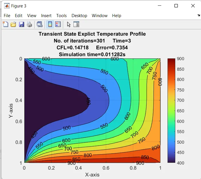
- Explict method coverges faster with less no. of iteration, of all the above method from steady as well as implict method