Week 9 - FVM Literature Review

Finite Difference Method (FDM):

• The computational domain is divided into node and then PDE ‘s are discretized and converted into algebraic solution and then solved using forward, backward and central differencing schemes for the nodes.
• FDM are easy to code and solve.
• FDM cannot be used where the nodes are not aligned along the cartesian coordinate system.
• FDM cannot be used to solve complex geometry problems.
• FDM does not conserve the properties as much as FVM.

Finite Volume Method (FVM):

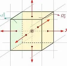
Fig. Control volume of cell with e as the cell centroid

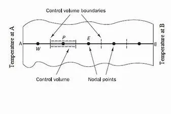
• The computational domain is divided into algebraic small volumes, as the governing equation is valid for this volume. hence it is valid at all control volume of the computational domain.
• FVM is comparatively difficult to code.
• As the FVM is solved by integrating throughout the volume of the domain hences it could be used to solve complex shaped geometry.
• The volume integrals in the PDE’s that contain divergence are converted to surface integrals.
• As the fluxes at the surfaces are evaluated, the flux entering each control volume being constant hence the properties are conserved better in FVM.

From the fig above while evaluating the point P the value at the point e and w are unknown hence the mathematical approximation method is required to compute the values at the surfaces. This approximation method is known as “Interpolation Schemes”.

Interpolation Schemes:

In the finite volume method, evaluation of surface and volume integrals sometimes requires the values of unknown variables other than the computational nodes of the control volume. These values are obtained by employing interpolation schemes.

Some interpolation schemes used in CFD are as follows:

1. Linear interpolation schemes
2. Upwind interpolation schemes
3. Linear upwind interpolation schemes
4. Quadratic Upwind interpolation for convective Kinematics (QUICK) schemes
5. Hybrid schemes
6. Total Variation Diminishing (TVD) schemes

Upwind interpolation schemes:

This scheme depends on the direction of the fluid flow

E.g. 1D linear convection problem

`(delU)/(delt) + alpha*(delU)/(delx) =0`

which describes a wave propagating along the x-axis with a velocity U. Consider a typical grid point i in the domain. In a one-dimensional domain, there are only two directions associated with point i– left (towards negative infinity) and right (towards positive infinity). If alpha is positive, the traveling wave solution of the equation above propagates towards the right, the left side of i is called upwind side and the right side is the downwind side. Similarly, if alpha is negative the traveling wave solution propagates towards the left, the left side is called downwind side and right side is the upwind side.

`(u^(n+1)(i) - u^n(i))/(Deltat) +alpha*(u^(n)(i) - u^n(i-1))/(Deltax) =0` for `alpha>0`

`(u^(n+1)(i) - u^n(i))/(Deltat) +alpha*(u^(n)(i+1) - u^n(i))/(Deltax) =0` for `alpha<0`

Flux value remains constant between the cell centroid and the cell faces; hence it is only 1^st order accurate. Even though the scheme is not that accurate but this is the most stable scheme for convection dominated flows. This method is generally used to generate an initial and stable solution.

Flux Limiters:

While calculating the variable gradient they tend to toggle and are not bounded to a particular value and keeps jumping, this occurs due to discontinuity due to shock occurring. Having a flux limiter will help to bound the gradient value there by giving a stable solution.

Flux limiters are also referred to as slope limiters because they both have the same mathematical form, and both have the effect of limiting the solution gradient near shocks or discontinuities. Flux limiter are used to limit the spatial derivates to realistic and meaningful values. They are used in high resolution scheme for solving problems described by PDEs and only come into operation when the sharp wave fronts are present.

Main idea is to tune the numerical flux of high order and low order schemes using the flux limiter function in such a way that the resulting scheme gives a high order accuracy in the smooth region of flow and sticks with the first order of accuracy in the vicinity of shock and discontinuity. Hence the flux limiter acts as a switch and helps in maintaining the slope of physical values in the vicinity of shock and discontinuity.