Week 10 - Simulating Combustion of Natural Gas.
AIM: To Perform the simulation analysis using methane-air fuel mixture and plot the variation of mass fraction of different species using line probes at different locations.
OBJECTIVE:
Part I
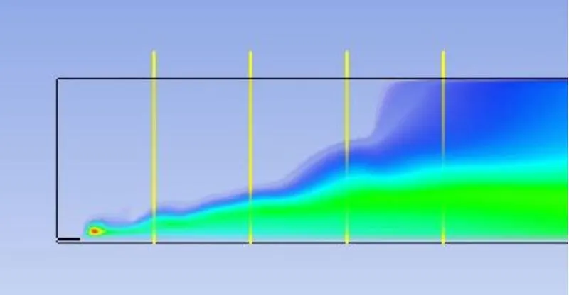
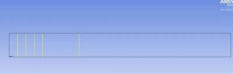
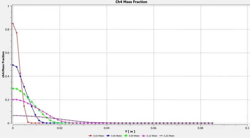
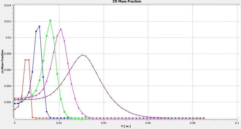
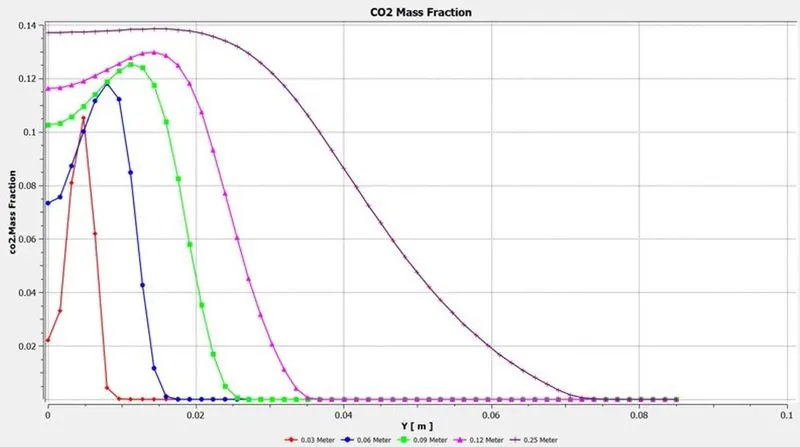
Perform a combustion simulation on the combustor model and plot the variation of the mass fraction of the different species’ in the simulation using line probes at different locations of the combustor as shown in Fig. You need to plot for CO2, H2O, CH4, N2, O2, NOx emissions & Soot formation.
Part II
As you must have observed from the above simulation, the Nox and soot is getting formed at the outlet of the combustor. Such formation has harmful effects on the environment and humans. The stringent government norms also demand the least formation of Nox and soot and to satisfy those requirements, you need to check the effect of adding the water in the fuel.
In this part, you need to add the water content in the fuel from 5% to 30% by mole and observe the effect of it on the results. It is necessary to provide line plots and contours to prove your claim.
THEORY AND EXPLANATION:
1. COMBUSTION:
Combustion, or burning, is a high-temperature exothermic redox chemical reaction between a fuel (the reductant) and an oxidant, usually, atmospheric oxygen, that produces oxidized, often gaseous products, in a mixture termed as smoke. Combustion does not always result in fire, because a flame is only visible when substances undergoing combustion vapourise, but when it does, a flame is a characteristic indicator of the reaction. While the activation energy must be overcome to initiate combustion (e.g., using a lit match to light a fire), the heat from a flame may provide enough energy to make the reaction selfsustaining. Combustion is often a complicated sequence of elementary radical reactions. Solid fuels, such as wood and coal, first undergo endothermic pyrolysis to produce gaseous fuels whose combustion then supplies the heat required to produce more of them. Combustion is often hot enough that incandescent light in the form of either glowing or a flame is produced. A simple example can be seen in the combustion of hydrogen and oxygen into water vapour, a reaction commonly used to fuel rocket engines. This reaction releases 242 kJ/mol of heat and reduces the enthalpy accordingly:
2H2(g) + O2(g) → 2H2O(g)
Combustion of an organic fuel in air is always exothermic because the double bond in O2 is much weaker than other double bonds or pairs of single bonds, and therefore the formation of the stronger bonds in the combustion products CO 2 and H2O results in the release of energy.
Stoichiometric combustion of a hydrocarbon in oxygen:
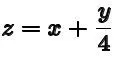
Generally, the chemical equation for stoichiometric combustion of a hydrocarbon in oxygen is:

Where,
For example, the stoichiometric burning of propane in oxygen is:

2. CHEMICAL KINETICS:
Chemical kinetics, also known as reaction kinetics, is the branch of physical chemistry that is concerned with understanding the rates of chemical reactions. It is to be contrasted with thermodynamics, which deals with the direction in which a process occurs but in itself tells nothing about its rate. Chemical kinetics includes investigations of how experimental conditions influence the speed of a chemical reaction and yield information about the reaction's mechanism and transition states, as well as the construction of mathematical models that also can describe the characteristics of a chemical reaction.
3. CHEMICAL REACTION MODEL:
Chemical reaction models transform physical knowledge into a mathematical formulation that can be utilized in computational simulation of practical problems in chemical engineering. Computer simulation provides the flexibility to study chemical processes under a wide range of conditions. Modelling a chemical reaction involves solving conservation equations describing convection, diffusion, and reaction source for each component species.
Series transport equation:

Ri is the net rate of production of species i by chemical reaction and Si is the rate of creation by addition from the dispersed phase and the user-defined source. Ji is the diffusion flux of species i, which arises due to concentration gradients and differs in both laminar and turbulent flows. In turbulent flows, computational fluid dynamics also considers the effects of turbulent diffusivity. The net source of chemical species i due to reaction, Ri which appeared as the source term in the species transport equation is computed as the sum of the reaction sources over the NR reactions among the species.
REACTION RATE MODELS:
A. LAMINAR FLOW RATE MODEL:
The laminar finite rate model computes the chemical source terms using the Arrhenius expressions and ignores turbulence fluctuations. This model provides the exact solution for laminar flames but gives inaccurate solution for turbulent flames, in which turbulence highly affects the chemistry reaction rates, due to highly non-linear Arrhenius chemical kinetics. However, this model may be accurate for combustion with small turbulence fluctuations, for example, supersonic flames. b. Eddy dissipation model:
The eddy dissipation model, based on the work of Magnussen and Hjertager, is a turbulent-chemistry reaction model. Most fuels are fast burning and the overall rate of reaction is controlled by turbulence mixing. In the non-premixed flames, turbulence slowly mixes the fuel and oxidizer into the reaction zones where they burn quickly. In premixed flames, the turbulence slowly mixes cold reactants and hot products into the reaction zones where the reaction occurs rapidly. In such cases, the combustion is said to be mixing-limited, and the complex and often unknown chemical kinetics can be safely neglected. In this model, the chemical reaction is governed by large-eddy mixing time scale. Combustion initiates whenever there is turbulence present in the flow. It does not need an ignition source to initiate the combustion. This type of model is valid for the non-premixed combustion, but for the premixed flames the reactant is assumed to burn at the moment it enters the computation model, which is a shortcoming of this model as in practice the reactant needs some time to get to the ignition temperature to initiate the combustion.
Factors affecting reaction rate:
- Nature of reactants
- Physical state
- Surface area of solid-state
- Concentration
- Temperature
- Catalysts
- Pressure
- Absorption of light
APPLICATIONS:
The mathematical models that describe chemical reaction kinetics provide chemists and chemical engineers with tools to better understand and describe chemical processes such as food decomposition, microorganism growth, stratospheric ozone decomposition, and the chemistry of biological systems.
These models can also be used in the design or modification of chemical reactors to optimize product yield, more efficiently separate products, and eliminate environmentally harmful byproducts.
When performing catalytic cracking of heavy hydrocarbons into gasoline and light gas, for example, kinetic models can be used to find the temperature and pressure at which the highest yield of heavy hydrocarbons into gasoline will occur can be used to find the temperature and pressure at which the highest yield of heavy hydrocarbons into gasoline will occur.
Chemical Kinetics is frequently validated and explored through modelling in specialized packages as a function of ordinary differential equation-solving (ODE-solving) and curve-fitting.
4. MASS FRACTION:
A mass fraction can also be expressed, with a denominator of 100, as a percentage by mass. It is one way of expressing the composition of a mixture in a dimensionless size; mole fraction (percentage by moles, mol%) and volume fraction (percentage by volume, vol%) are others. When the prevalences of interest are those of individual chemical elements, rather than of compounds or other substances, the term mass fraction can also refer to the ratio of the mass of an element to the total mass of a sample. In these contexts, an alternative term is a mass per cent composition. The mass fraction of an element in a compound can be calculated from the compound's empirical formula or its chemical formula.
5. NITROGEN OXIDE (NOX) EMISSIONS:
Nitrogen dioxide is an irritant gas, which at high concentrations causes inflammation of the airways. When nitrogen is released during fuel combustion it combines with oxygen atoms to create nitric oxide (NO). This further combines with oxygen to create nitrogen dioxide (NO2). Nitric oxide is not considered to be hazardous to health at typical ambient concentrations, but nitrogen dioxide can be. Nitrogen dioxide and nitric oxide are referred to together as oxides of nitrogen (NOx).
NOx gases react to form smog and acid rain as well as being central to the formation of fine particles (PM) and ground-level ozone, both of which are associated with adverse health effects.
6. SOOT FORMATIONS:
Soot forms when hydrocarbon fuels such as oil, natural gas, and wood are burned. Soot particles form when gaseous molecules are heated to high temperatures, and they don't easily turn back into gaseous molecules the way water droplets do when they are heated. Soot as an airborne contaminant in the environment has many different sources, all of which are results of some form of pyrolysis. They include soot from coal-burning, internal-combustion engines, power-plant boilers, hog-fuel boilers, ship boilers, central steam-heat boilers, waste incineration, local field burning, house fires, forest fires, fireplaces, and furnaces. These exterior sources also contribute to the indoor environment sources such as smoking of plant matter, cooking, oil lamps, candles, quartz/halogen bulbs with settled dust, fireplaces, exhaust emissions from vehicles, and defective furnaces.
Types of combustion simulation:
- Non-premixed combustion (Direct injection, Late injection)
- Premixed Combustion (Carburetor)
- Partially premixed.
NON-PREMIXED COMBUSTION:
In non-premixed combustion, fuel and oxidizer enter the reaction zone in distinct streams. This is in contrast to premixed systems, in which reactants are mixed at the molecular level before burning. Examples of non-premixed combustion include pulverized coal furnaces, diesel internal-combustion engines, and pool fires.
Direct injection is used in heavy-duty vehicles. Similar to diesel engines, high thermal efficiency and power density are maintained in such direct injection natural gas engines. In such engines, natural gas is injected directly into the combustion chamber. Then the gas mixes with the high-pressure air in the combustion chamber and combustion occurs. Due to the nonpremixed nature of the combustion occurring in such engines, a non-premixed combustion model of ANSYS FLUENT can be used to simulate the combustion process. Premixed Combustion:
In pre-mixed combustion, fuel and oxidizer are mixed at the molecular level prior to ignition. Combustion occurs as a flame front propagating into the unburnt reactants. Examples of premixed combustion include aspirated internal combustion engines, lean-premixed gas turbine combustors, and gas-leak explosions.
Premixed combustion is difficult to model that non-premixed combustion. The reason for this is that premixed combustion usually occurs as a thin, propagating flame that is stretched and contorted by turbulence. For subsonic flows, the overall rate of propagation of the flame is determined by both laminar and turbulent eddies. The laminar flame speed is determined by the rate that species and heat diffuse upstream into the reactants and burn. To capture the laminar flame speed, the internal flame structure would need to be resolved, as well as the detailed chemical kinetics and molecular diffusion processes. Since practical laminar flame thicknesses are of the order of millimeters or smaller, resolution requirements are usually unaffordable.
The effect of turbulence is to wrinkle and stretch the propagating laminar flame sheet, increasing the sheet area and in turn the effective flame speed. The large turbulent eddies tend to wrinkle and corrugated the flame sheet while the small turbulent eddies if they are smaller than the laminar flame thickness, may penetrate the flame sheet and modify the laminar flame structure.
PARTIALLY PRE-MIXED COMBUSTION:
Partially premixed combustion systems are premixed flames with non-uniform fuel-oxidizer mixtures. Such flames include premixed jets, discharging into a quiescent atmosphere, lean-premixed combustors with diffusion pilot flame and cooling air jets, and imperfectly mixed inlets.
The partially premixed model in FLUENT is a simple combination of the non-premixed model and the premixed model. The premixed reaction progress variable determines the position of the flame front. Behind the flame front, the mixture is burnt and the equilibrium or laminar flamelet mixture fraction solution is used. Ahead of the flame front the species mass fractions, temperature, and density are calculated from the mixed but unburnt mixture fraction. Within the fame, a linear combination for the unburnt and burnt mixtures is used.
B. BASED ON PHASE:
- Fluid phase:- In this model, the fuel is in the liquid phase and combustion reactions are happening at the volume of thechamber.
- Wall:- In this model, the combustion reactions are done at the surface of the combustion chamber.
- Particles:- In this model, the reactions are being performed at the surface of the particles.
- Porous regions:- In this model, the reactions are being performed in the porous regions.
COMBUSTION SOURCE CALCULATION:
FINITE RATE CHEMISTRY:
This model derives ODE for all species and solves them. It results in accurate solutions but the computational time required to solve the ODE is increased as the number of species involved is more.
MIXING BASED MODEL:
EDDY DISSIPATION MODEL:
In this model, the combustion takes place when there is a presence of turbulence, hence it does not require any heat source to initiate the combustion reaction. This model is valid for non-premixed fuel mixture.
FINITE RATE EDDY DISSIPATION MODEL:
It is the combination of both finite rate chemistry and the eddy dissipation model. In this model, the kinetic rate is calculated in addition to the reaction rate calculated from the eddy dissipation model.
Then the slowest reaction is chosen.
- If turbulence is low, the species mixing rate is low, this limits the reaction rate.
- If turbulence is high, the kinetic rate is low, this limits the reaction rate.
GEOMETRY:
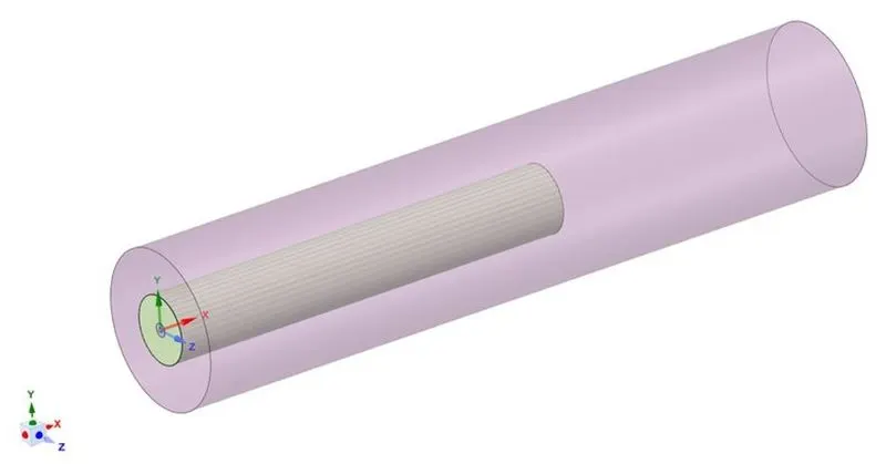
1. Upload the combustor model onto SpaceClaim, since it is a 3D model and we are only interested in the 2D geometry of thecombustor. Therefore, we need to split the body by 3/4th and select the plane XY plane region of geometry since we are using the axisymmetric condition. 3D model of the combustor:
2. The geometry clean-up is done for the burner 3D model. As it required to create 2D model from provided geometry of burner. The model will directly open in space-claim design modeler and planes are created at the center point of geometry which is shown in below
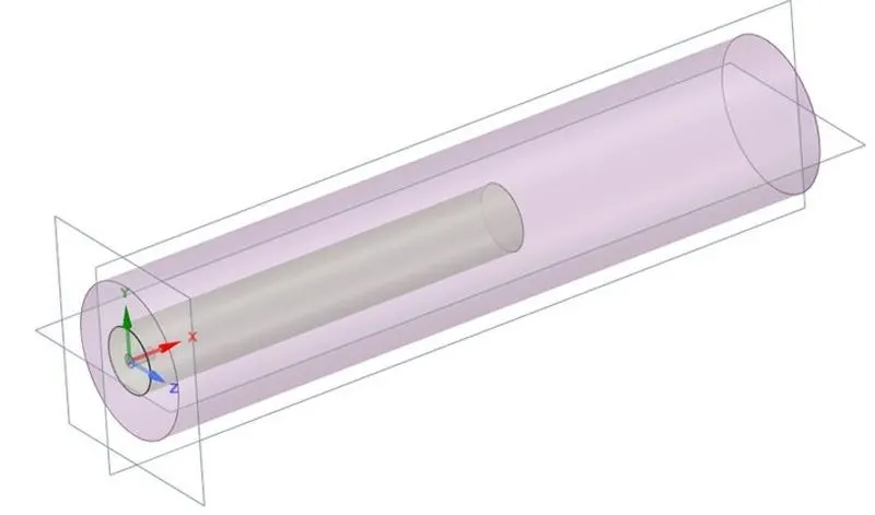
3. As for 2D Axisymmetric model it required to cut in quarter model and then the face of that quarter section is copied and pasted in new design. Before copying the face of quarter section, it is required to combine the two section of geometry which are present in whole assembly. Both the geometry instead of fuel opening area can be treated as one body. After creation plane the split body option from space-claim design tab is used to cut the body in half first parallel to XY plane and then it need to be cut parallel to ZX plane.
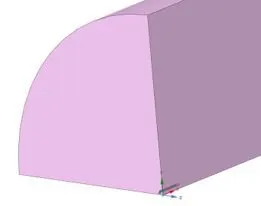
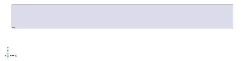
The front face of geometry can be used for simulation. To have the face for simulation it is necessary to select the face and copy it. After copying the face from geometry, it has to be pasted in new design which can be made from File>New>Design option. The geometry must be pasted only in XY plane for the sake of Axisymmetric approach. Figure shows the final geometry for simulation.
MESHING:
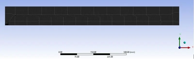
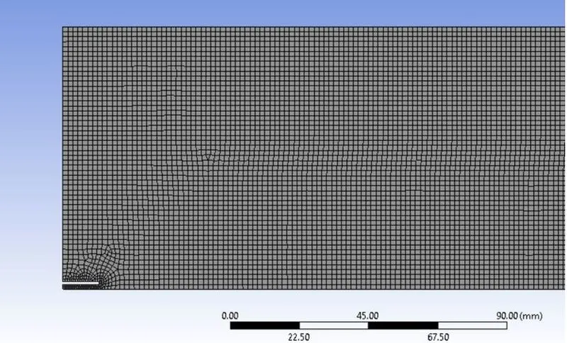
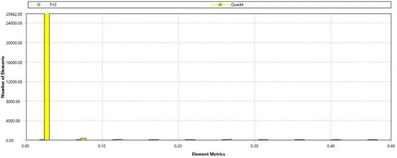
The type of element which is used for meshing is Quad 4. Because of simplicity of geometry and accuracy of solution required, it is best practice to go with quadrilateral elements. The method used for the meshing is Automatic method in which Quadrilateral dominant method has been used. In the geometry there are some irregularity which cause element to reshape in zone of vicinity. The proximity size function is used for providing element in the smaller zones of geometry. The proximity size function requires number cell across the gap in geometry. As there is only one possible gap in geometry near the left hand bottom side and it is necessary to create more number of element near the fuel inlet. The number of cell in the gap is provided as 3 and the element size of 1.6mm is used for whole geometry.
MESH QUALITY:
The element quality for overall mesh setup is in best condition. The maximum skewness for the mesh is 0.48 and the maximum aspect ratio 1.62. The orthogonal quality of mesh is just opposite to skewness.
CASE SETUP:
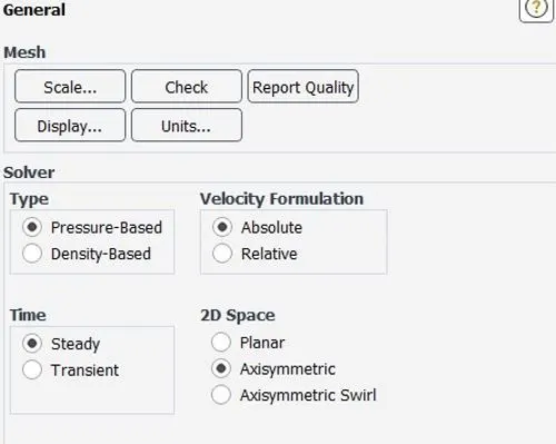
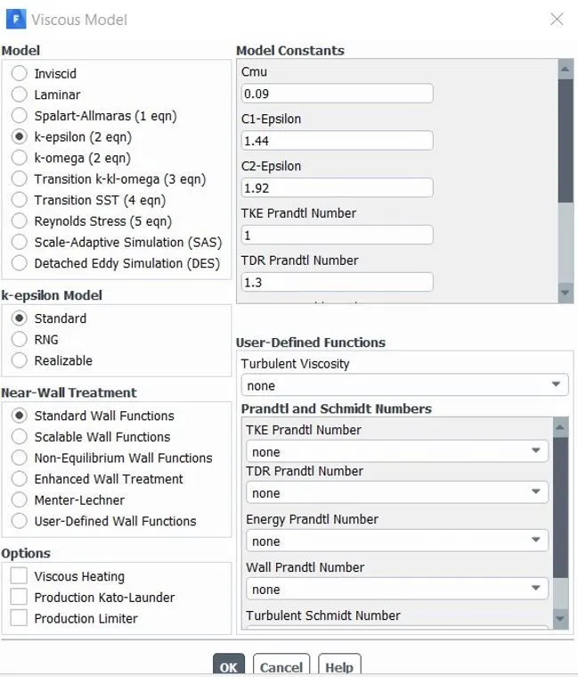
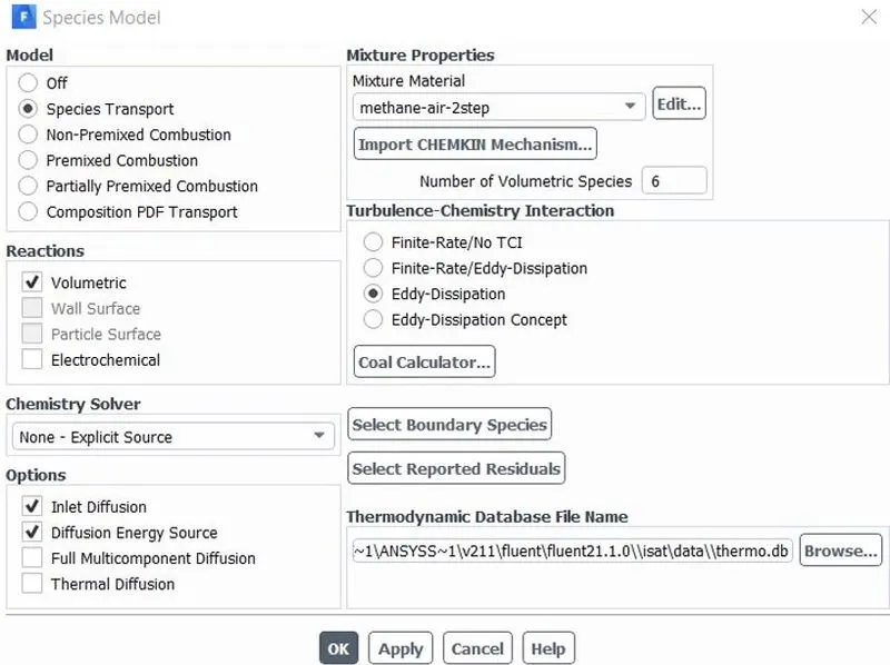
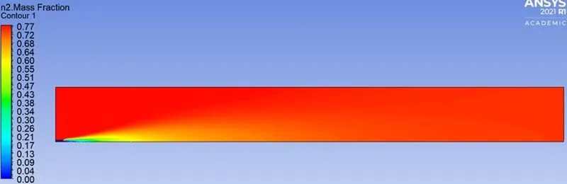
After completing the viscous model selection, the species model can be selected from the model of FLUENT in outline view or can be also select from physics tab > models. As the species model turn on, the energy equation will get turn on automatically. Energy model use to determine the temperature generated during the reaction in species transport equation. In species model, species transport option has to be selected followed by volumetric reaction. The mixture properties should be select one at a time. If user has select any other mixture properties model rather than given one, then that setup need to be reset and again whole process has to be followed accordingly. The mixture model which is used for simulation is ‘methane-air2step’ in which number of volumetric species are six i.e. CO2, H2O, CH4, N2, O2 and CO. As state earlier this model is governed by effect of turbulence hence Eddy dissipation turbulence-chemistry interaction is selected.
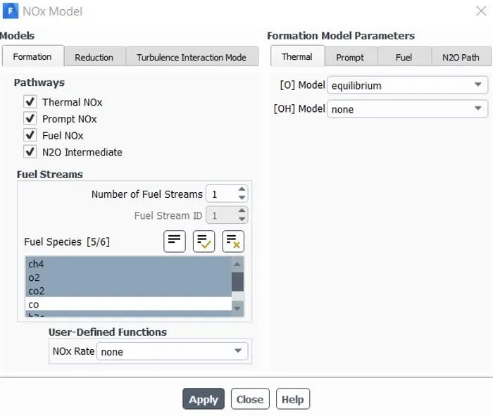
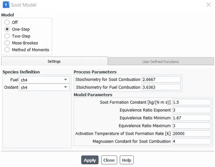
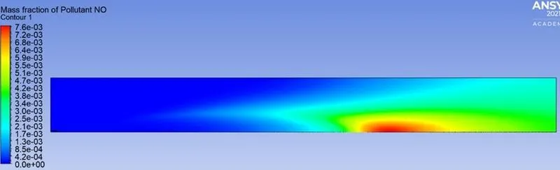
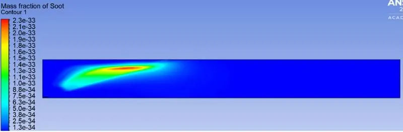
Similar to species model setup, NOx and soot model has to be done accordingly. As discussed earlier the NOx can be produce due to high temperature and rich fuel mixture, hence all the pathways which can track the generation of NOx are activated for the simulation. Similarly, the soot model is also activated in which one-step soot model is used for the tracking of soot generation during the combustion process.
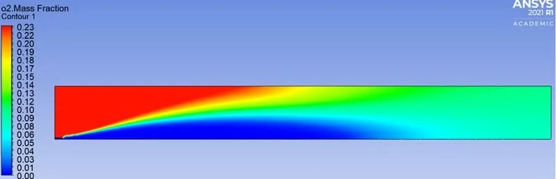
The boundary conditions which are used for this simulation are velocity inlet and pressure outlet with an axis for Axisymmetric condition. There are two inlets for this simulation. The first velocity inlet is for air which is flowing inside the burner at the speed of 0.5m/sec. The Air is entering at atmospheric pressure inside burner and at 300 kelvin temperature. In species tab of air inlet, it is required to provide information about how much of oxygen is entering in the burner. The 0.23 mass fraction of O2 is coming with air for the reaction purpose.
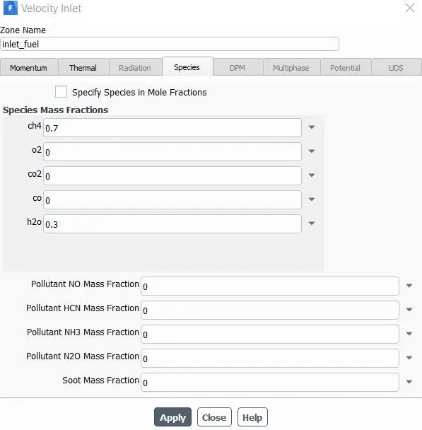
Similarly, for the fuel inlet the momentum boundary conditions are consider are velocity inlet with the value of 80m/sec. The fuel is also entering at atmospheric pressure and 300 kelvin temperature. The most important part of fuel inlet is the specification of species for the simulation. In the species tab of fuel inlet boundary condition the mass fraction of Fuel is defined as 1 of CH4. The information about fuel inlet boundary condition.
Other than this boundary condition, the pressure outlet boundary condition is kept similar and axis should be put as axis as per the defined by FLUENT automatically.
RESULTS:
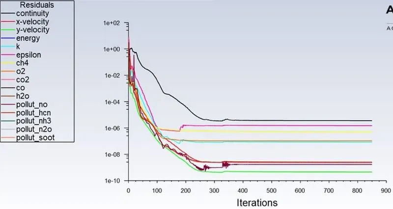
Residual Plot
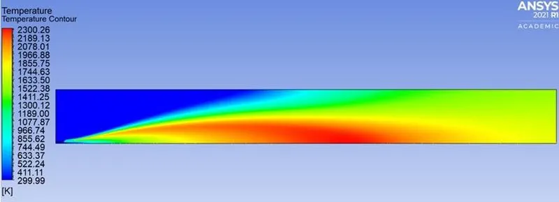
Temperature plot
Mass fraction of CH4
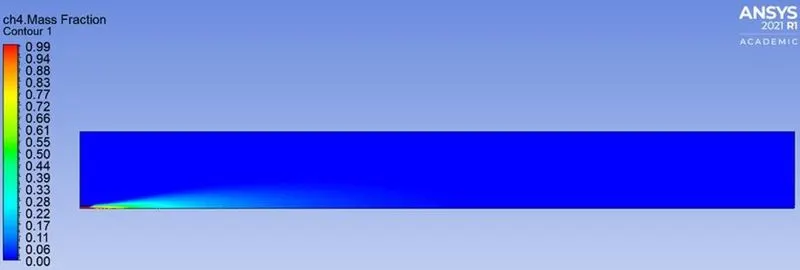
Mass Fraction CO
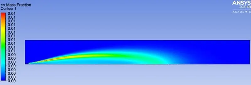
Mass Fraction of CO2
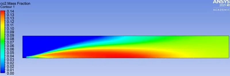
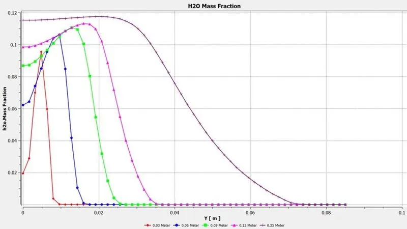
Mass Fraction of H2O
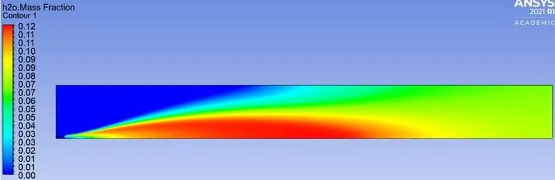
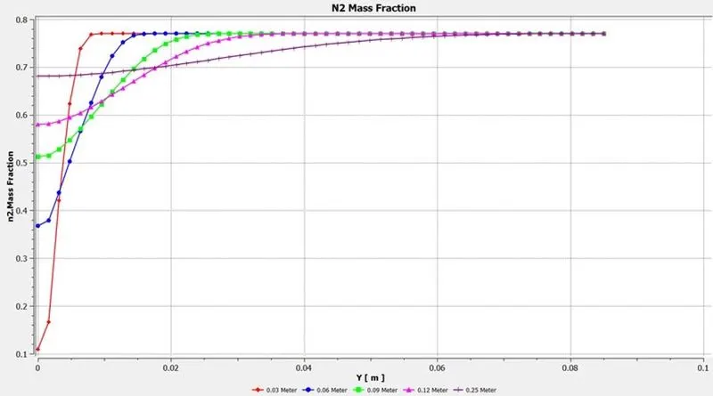
Mass Fraction of N2
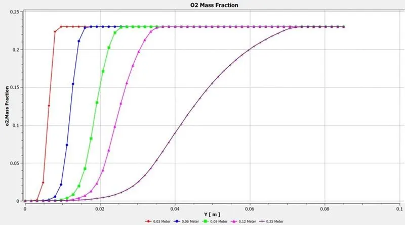
Mass Fraction of O2
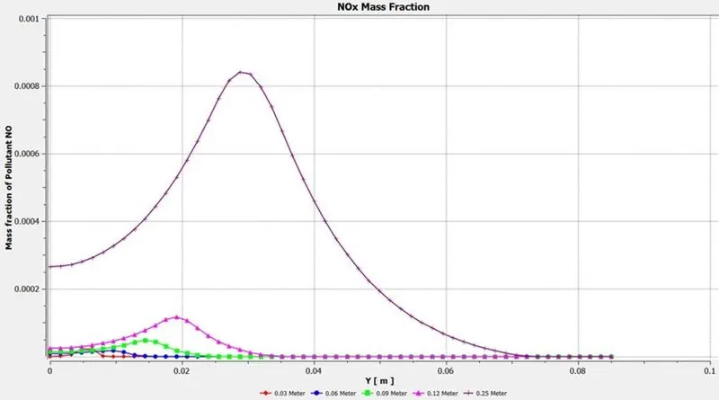
Mass fraction of NOx
Mass Fraction of Soot
Line Plots for graphs
Graph of CH4
Graph of CO
Graph of CO2
Graph of H2O
Graph of N2
Graph of O2
Graph of NOx
Graph of Soot
CASE1: OXYGEN 5%
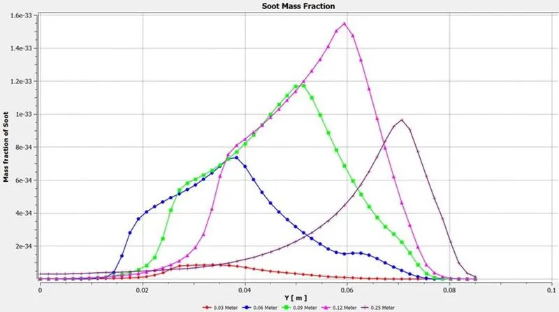
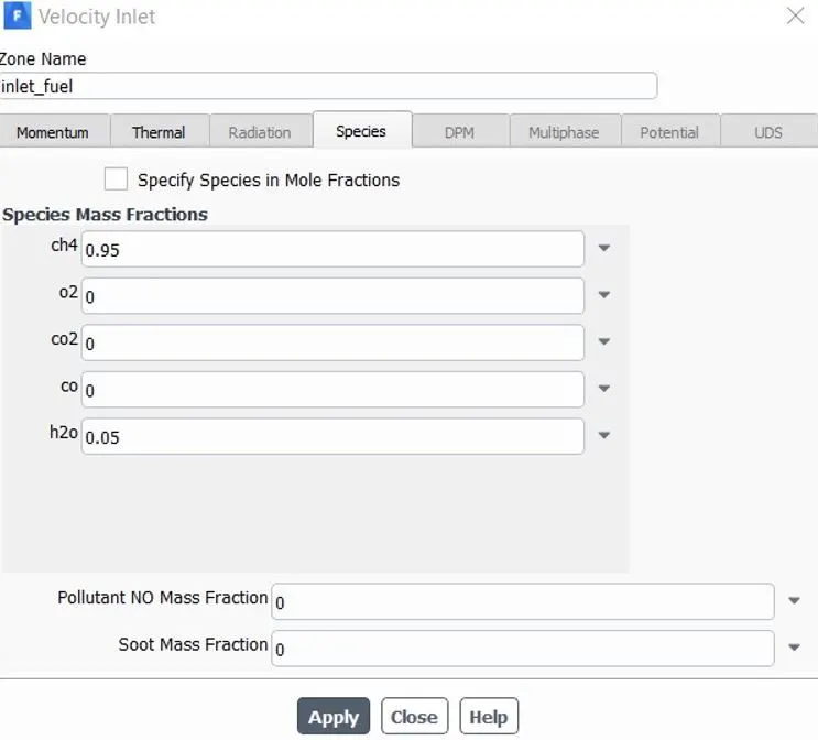
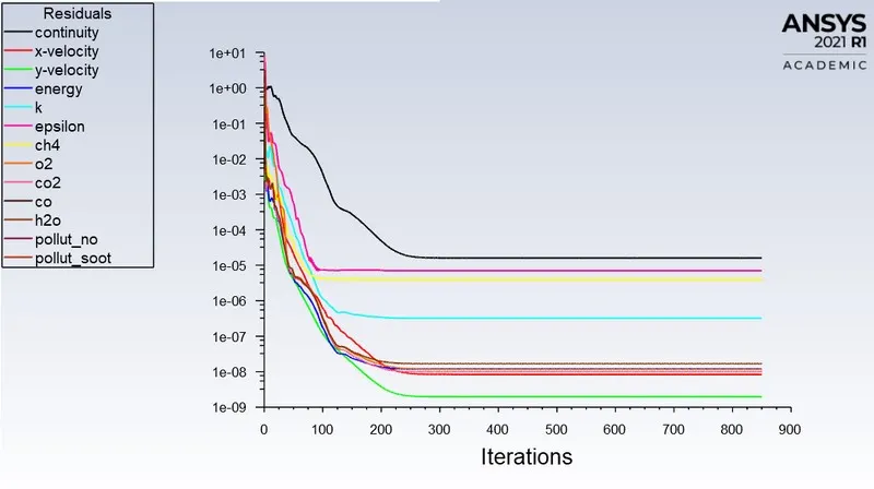
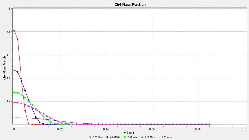
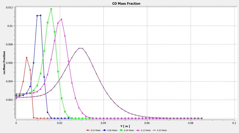
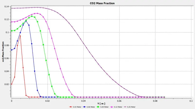
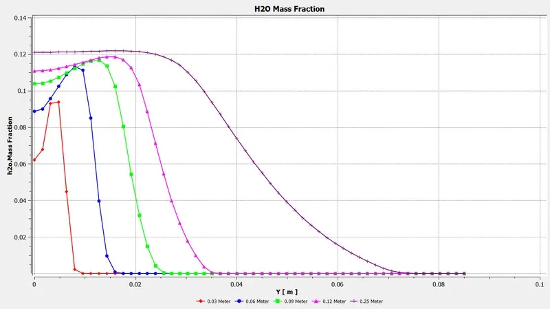
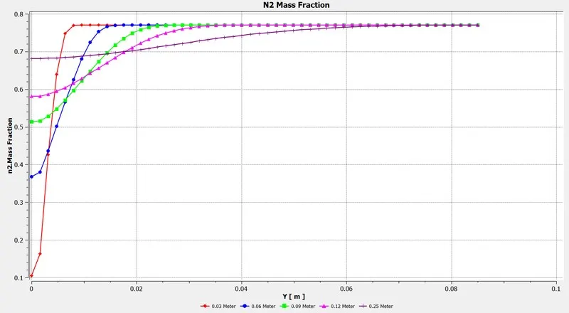
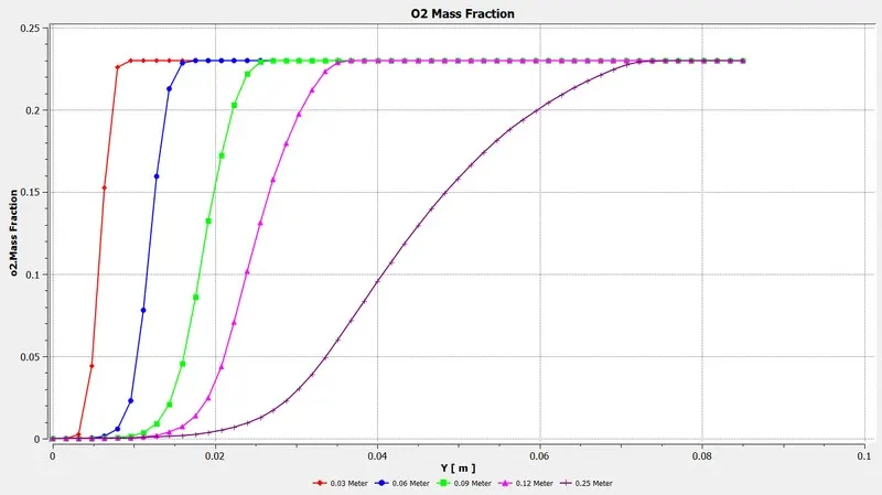
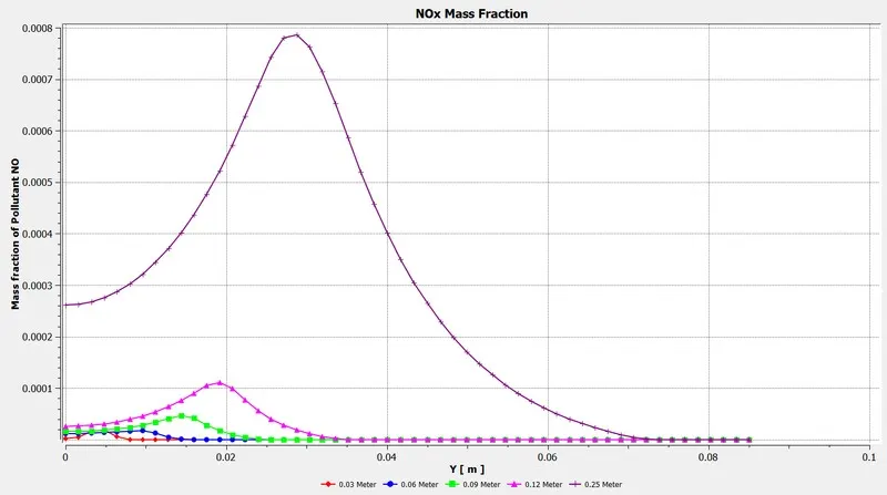
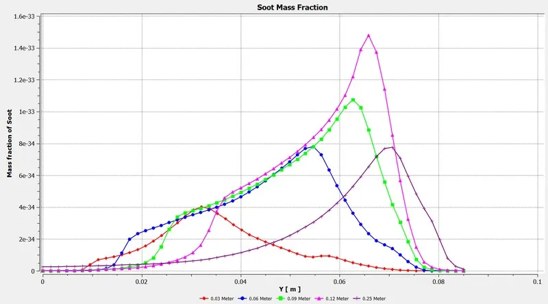
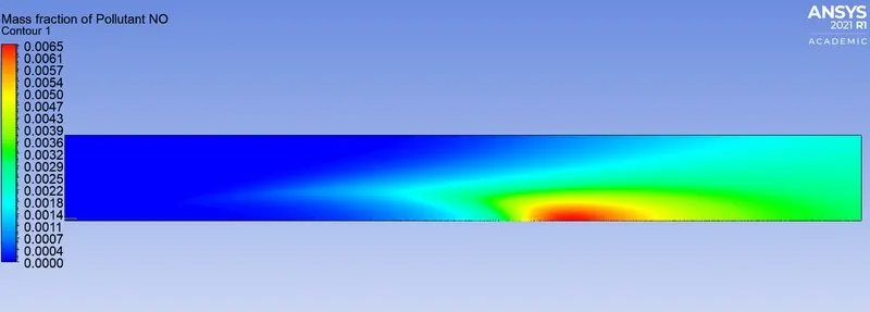
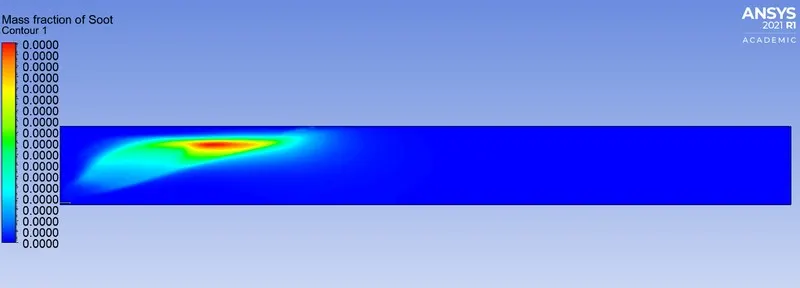
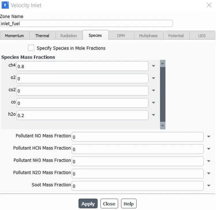
In baseline mesh setup it can be seen that there is proportion of NOx and soot is generated inside the burner. the location of NOx is toward the outlet is more and soot formation is done near the air inlet. To lower the NOx and soot formation in burner the fuel is mixed with Water vapour which entering from same inlet location. For this case only 5% of water is made to mix with fuel and flow at 80m/sec velocity. As the Mass fraction of water is increased in fuel inlet consequently the mass fraction of fuel has to be decrease. The mass fraction of water in this case will be 0.05 whereas mass fraction of fuel will be 0.95.
Residual plot
Temperature plot
Graph of CH4
Graph of CO
Graph of CO2
Graph of H2O
Graph of N2
Graph of O2
Graph of NOx
Graph of Soot
Mass Fraction of NOx
Mass Fraction of Soot
CASE2: OXYGEN 10%
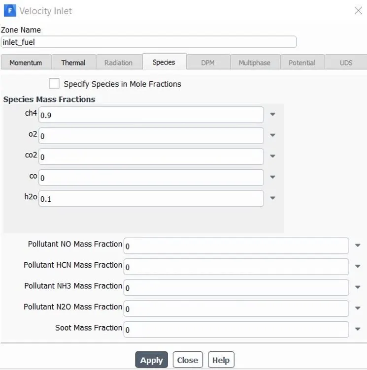
In Case 2 the percentage of oxygen is increased by 5% again. The specification of mass fraction of fuel.
Residual plot
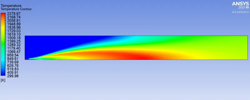
Temperature plot
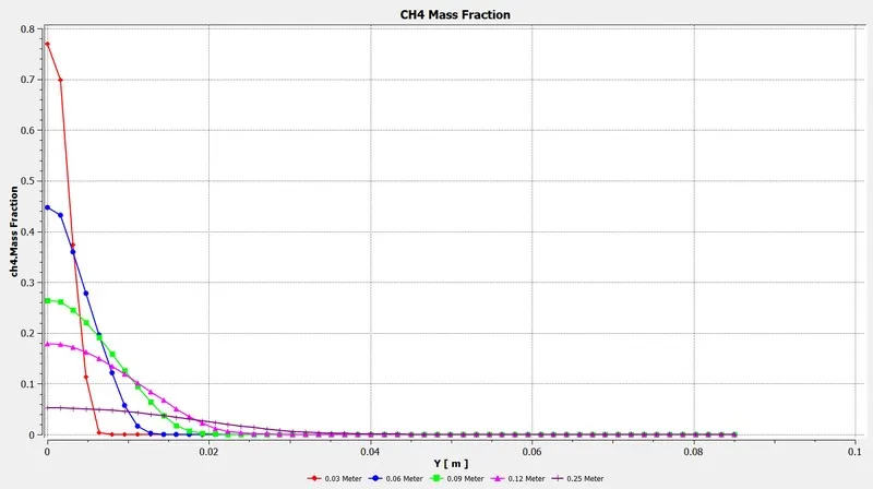
Graph of CH4
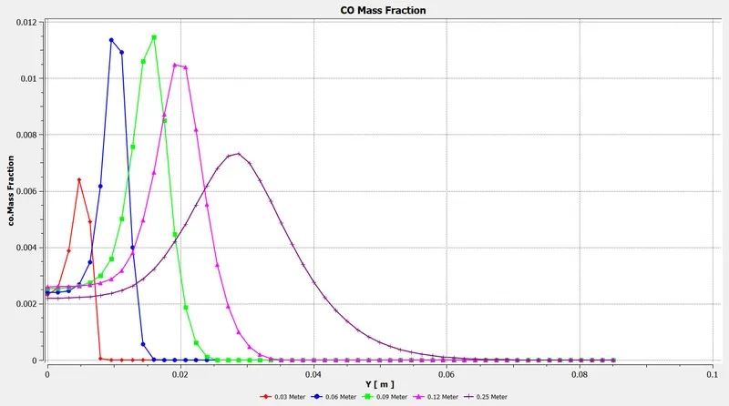
Graph of CO
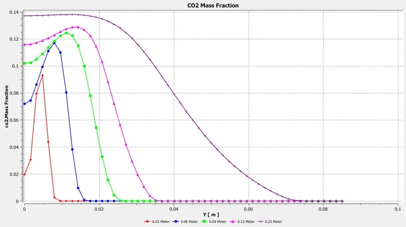
Graph of CO2
Graph of H2O
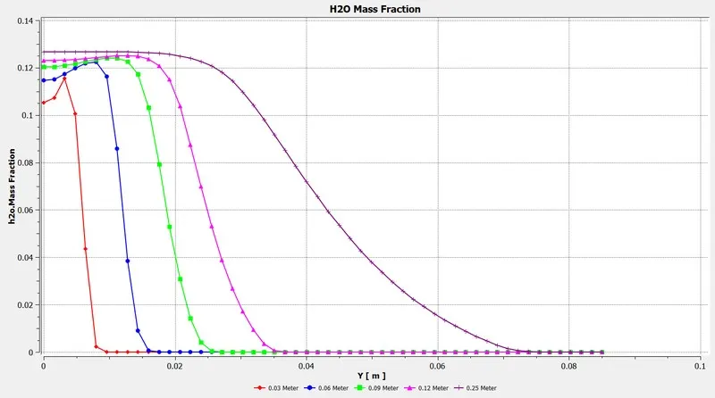
Graph of N2
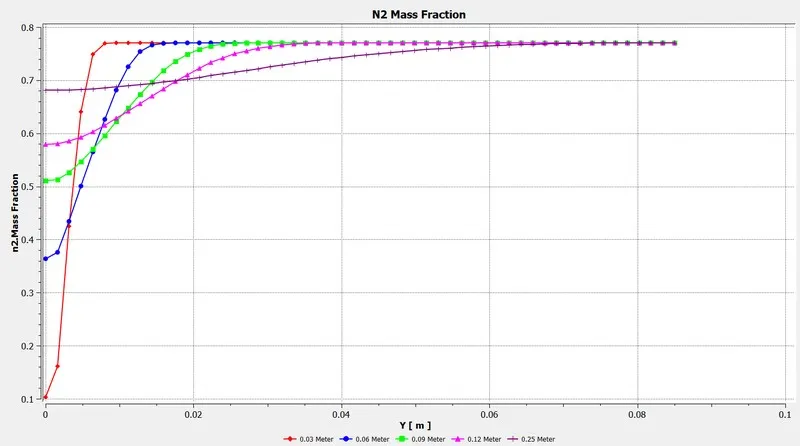
Graph of O2
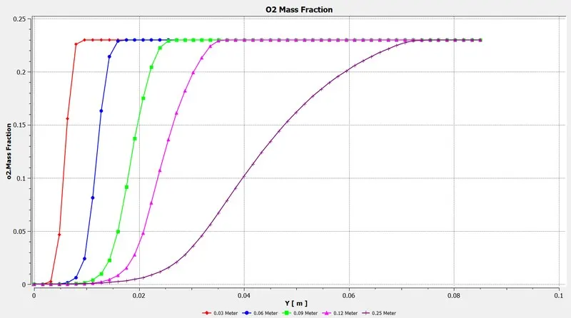
Graph of NOx
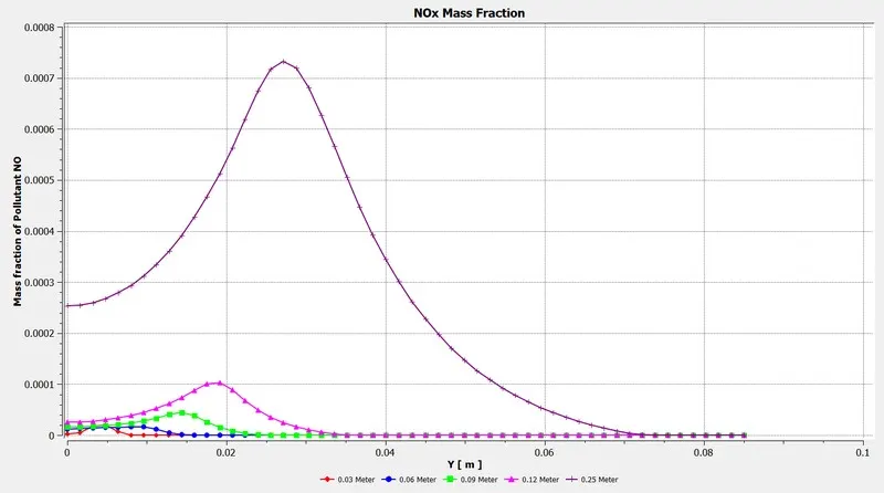
Graph of Soot
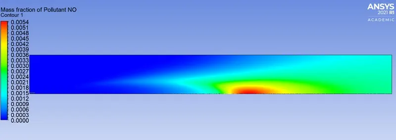
Mass Fraction of NOx
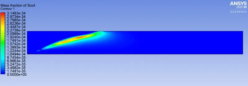
Mass Fraction of Soot
CASE3: OXYGEN 20%
In Case 3 the percentage of oxygen is increased by 10% again. The specification of mass fraction of fuel and water.
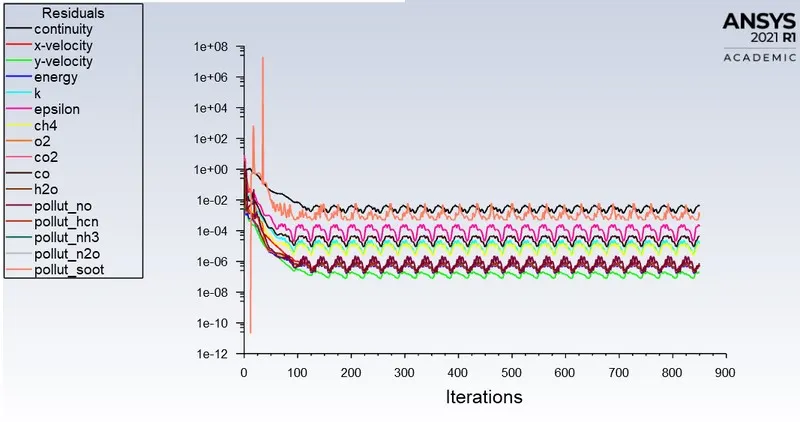
Residual plot
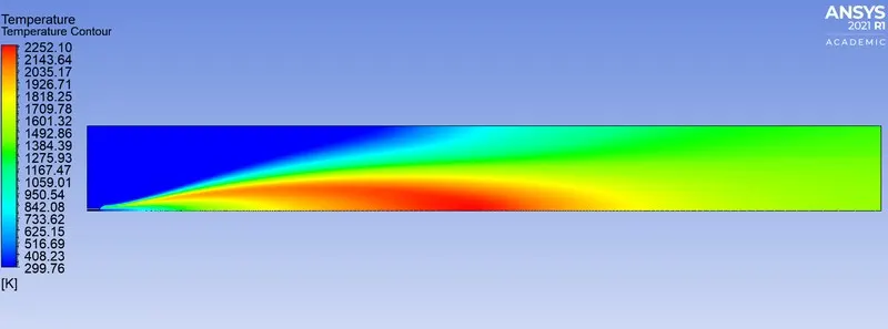
Temperature plot
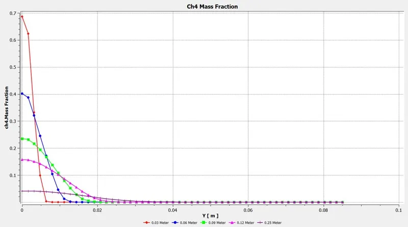
Graph of CH4
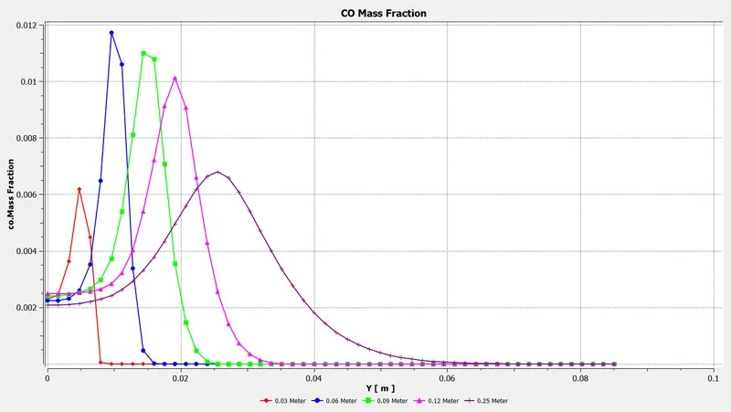
Graph of CO
Graph of CO2
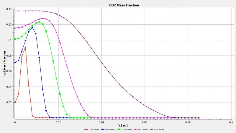
Graph of H2O
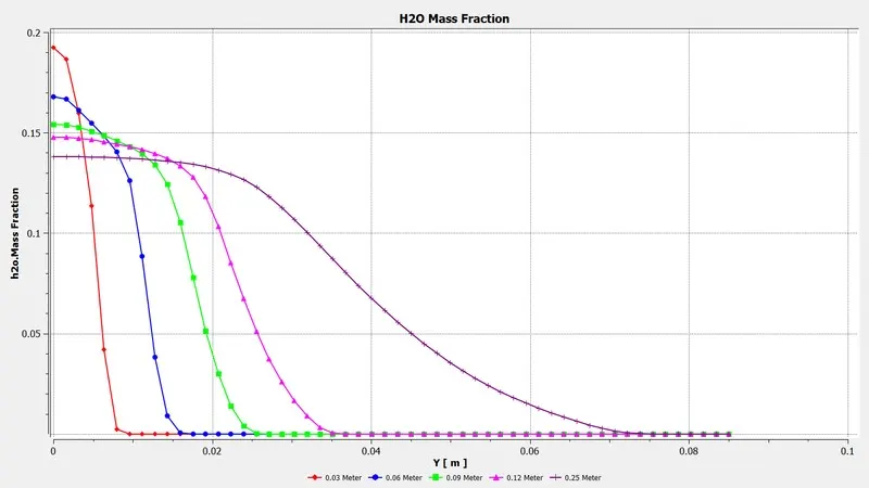
Graph of N2
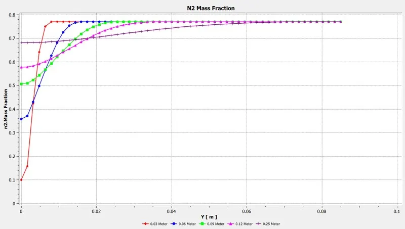
Graph of O2
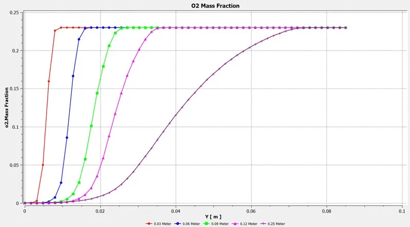
Graph of NOx
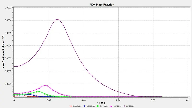
Graph of Soot
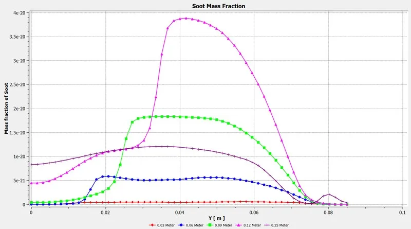
Mass Fraction of NOx
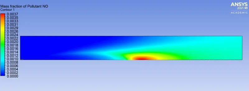
Mass Fraction of Soot
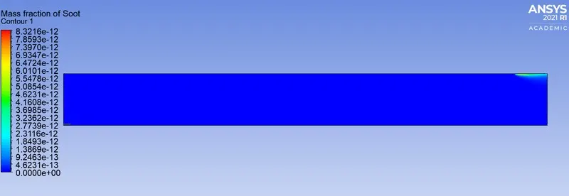
CASE4: OXYGEN 30%
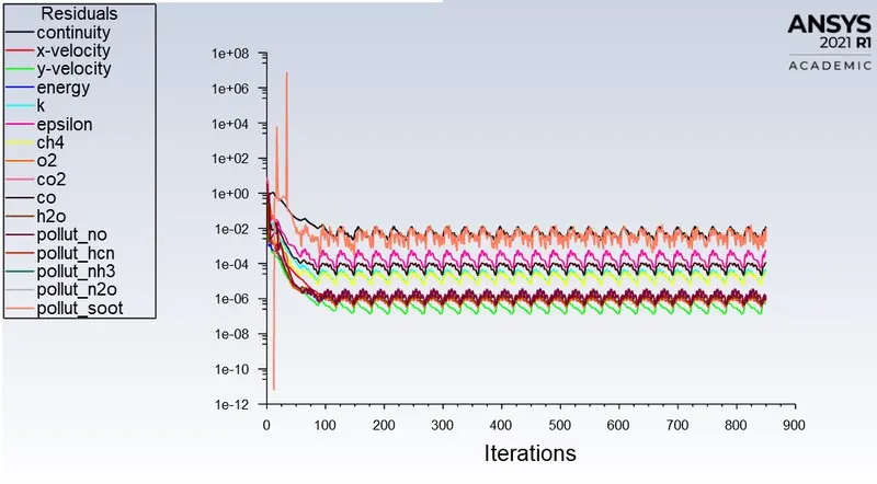
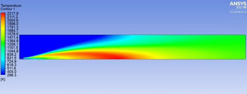
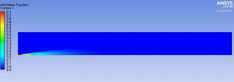
In Case 4 the percentage of oxygen is increased by 10% again. The specification of mass fraction of fuel and water.
Residual plot
Temperature Contour
Mass Fraction of CH4
Mass Fraction of CO
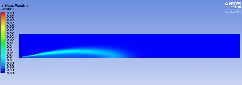
Mass Fraction of CO2
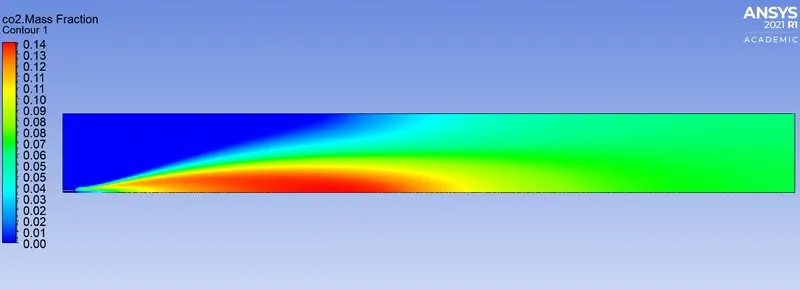
Mass Fraction of H2O
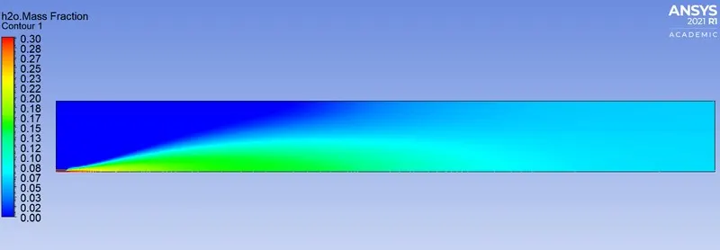
Mass Fraction of N2
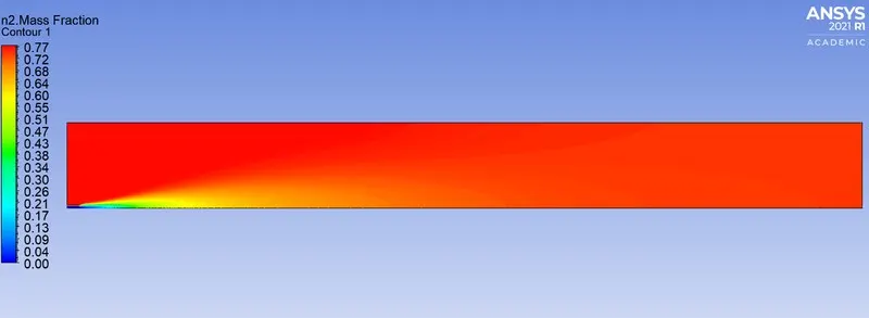
Mass Fraction of O2
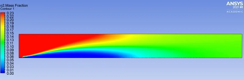
Mass Fraction of NOx
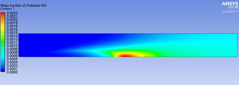
Mass Fraction of Soot
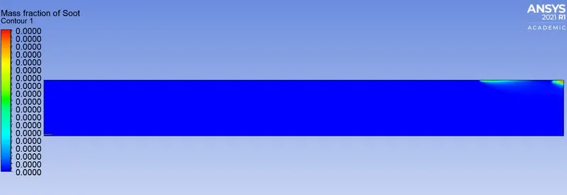
Graph of CH4
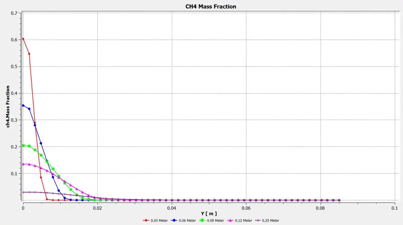
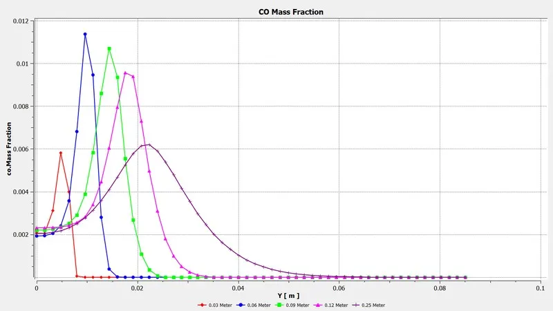
Graph of CO
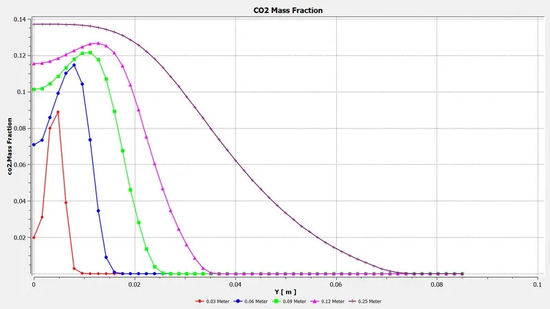
Graph of CO2
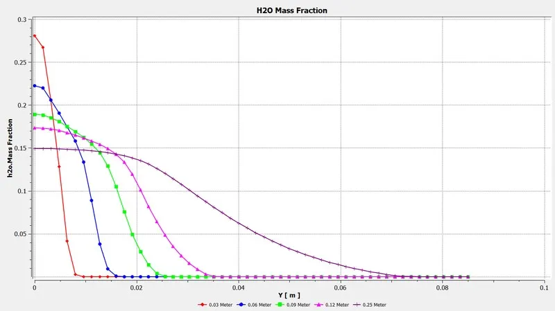
Graph of H2O
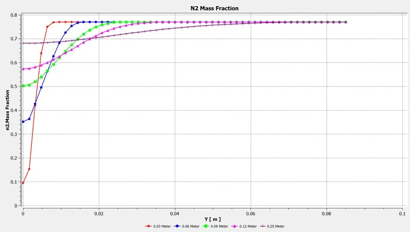
Graph of N2
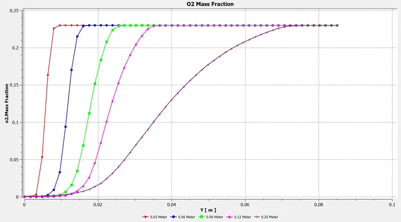
Graph of O2
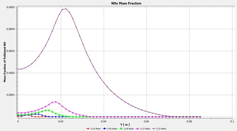
Graph of NOx
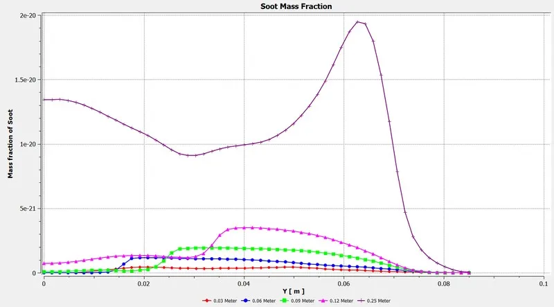
Graph of Soot
RESULT TABLE:
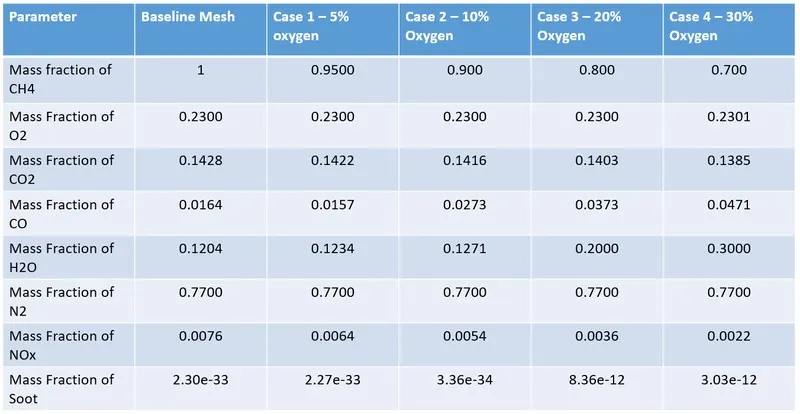
Results of all cases of simulation.
conclusion:
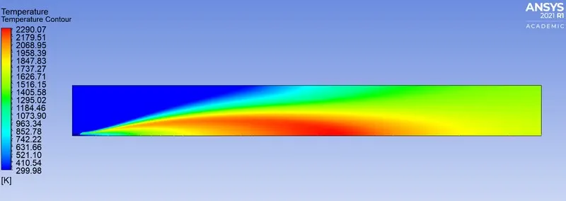
- In baseline mesh setup in which the whole amount of CH4 is present for as the fuel the amount of soot and NOx is greater as compared to other cases. Also the maximum temperature is about 2300 K.
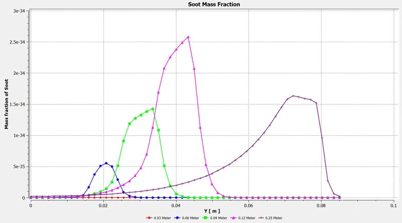
- In next cases where the water is added with fuel in respect of 5% to 30% there is reduction of NOx by certain amount. For case 1 the reduction of NOx is about 15.78%. For case 2 same reduction of NOx is 28.94%. For case 3 the NOx reduction is 52.64% whereas for case 4 the NOx reduction is about 71.05%. Hence adding the water with fuel is considerably decreasing the NOx emissions from the exhaust products.
- Similar to NOx, from the result table it can be seen that the mass fraction of CO2 is also decreasing as water percentage is increasing. The Mass fraction of N2 is almost constant for all the cases which means the flame instability for the burner is almost constant for all the cases of combustion.
- In case of soot formation, it can see that, mass fraction of soot is decreasing for case 1 and 2 but for case 3 and 4 it has increased. After checking the Mass fraction of soot contour for all the cases, it is evident that soot formation from case 1 to 4 is unbalanced but the amount of soot formation is significantly lowered for case 3 and 4. It is seen that from case 3 and 4 contour of mass fraction of soot, the formation of soot is nearer toward the outlet of burner which is common practice of soot to deposited at the outlet.
- From the whole simulation it concluded that providing water with fuel will reduce the harmful exhaust emission such as NOx and Soot.