Week 10 - Simulating Combustion of Natural Gas.

The aim, Introduction, Theory

The objective of the above simulation is to understand combustion in a combustor model using mass fractions of different species. The fuel used in this case will be Methane adn there will be two scenarios.

Case I- Perform a combustion simulation on the combustor model and plot the variation of the mass fraction of the different species’ in the simulation using line probes at different locations of the combustor as shown in Fig. You need to plot for CO2, H2O, CH4, N2, O2, NOx emissions & Soot formation.

Case II- From the above simulation, the Nox and Soot is getting formed at the outlet of the combustor. Such formation has harmful effects on the environment and humans. The stringent government norms also demand the least formation of Nox and soot and to satisfy those requirements, you need to check the effect of adding the water in the fuel.

In this part, you need to add the water content in the fuel from 5% to 30% by mole and observe the effect of it on the results. It is necessary to provide line plots and contours to prove your claim.

Combustion is a combination of physical and chemical process where oxygen reacts to liberate heat under certain physical conditions such as high temperature or high pressure. While reacting combustion forms certain by products which maybe soot or NOx. Soot and NOx are the main contributors to pollution leading to climate change. Modelling these chemical phenomenon and processes can help us reduce by product emissions and reduce pollution in general. Modelling of combustion can be comparitively cheaper and easy with CFD.

Solving & Modelling approach

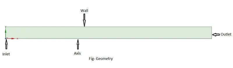
The geometry is so aligned that it can be qualified for axisymmetric simulation. The reason for choosing an axisymmetric geometry is due to the fact that simulating actuall 3D geometry would be very costly with bit complicated data. Moreover we can deduce similar results from a 2D geometry. The geometry here used is a draw with appropriate dimensions.

The next process in workflow is Meshing of the geometry. The geometry is fairly simple and we can use unifom meshing in order to get good quality mesh. I have used triangle method of cell creation. The element size is set at 10 mm. The opening of the combustor or the inlet is very small so the mesh becomes little coarse near the inlet. In mesh setting, capture proximity is turned on with proximity minimum size of 0.1 mm and Num cell across gap set to 3.

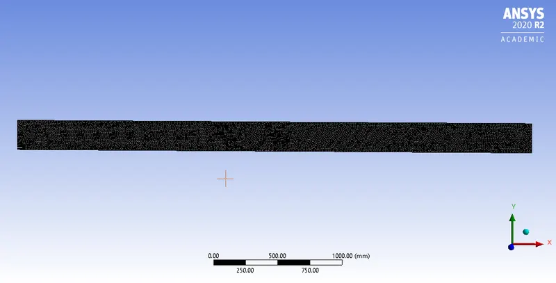
Fig.2- Mesh

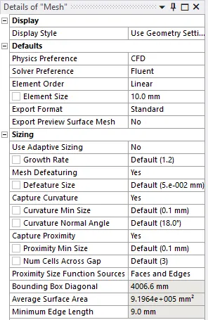
Fig.3- Mesh setting

Pre-processing and solver setting:

Combustion can be a complicated process to simulate, but for the above case we can use Pressure based solver. We check axisymmetric 2D space as the whole body can be completed once we use 360 degree of the 2D geometry. Specific models are to be checked as we are going to simulate for soot and NOx emissions among various other parameters. There is turbulence which should be taken into consideration for that I have used standard k-epsilon viscous model. The solver settings and pre processing details are shown below.

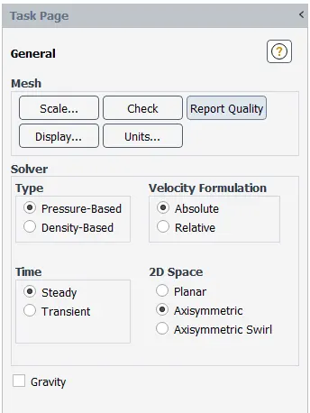
Fig.4- Solver settings

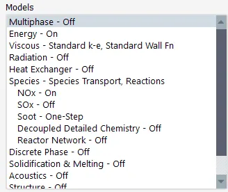
Fig.5- Solution model settings

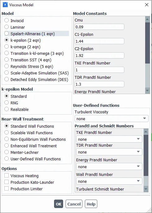
Fig.6- Viscous model settings

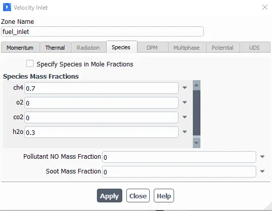
Fig.7- Inlet condition

Results:

Case I

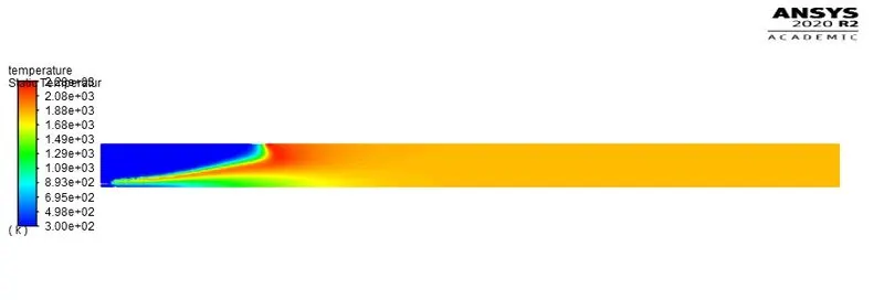
Fig.8- Temperature contour for case I simulation

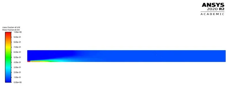
Fig.9- Contours for mass fraction of CH4

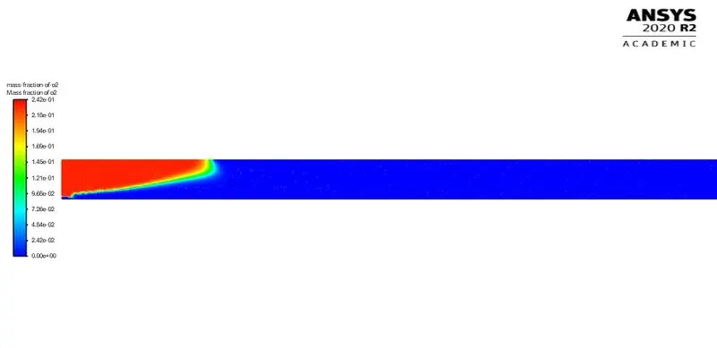
Fig.10- Contours for mass fraction of CO2

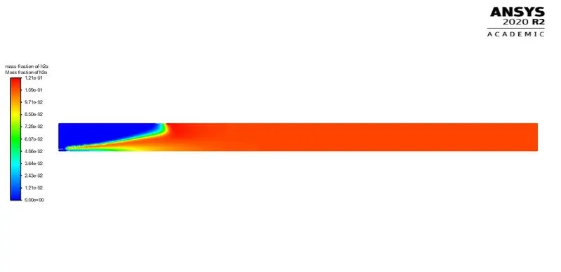
Fig.11- Contours for mass fraction of H2O

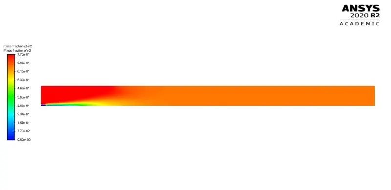
Fig. 12- Contours for mass fraction of N2

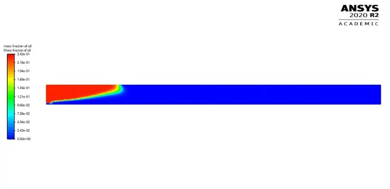
Fig.13- Contours for mass fraction of O2

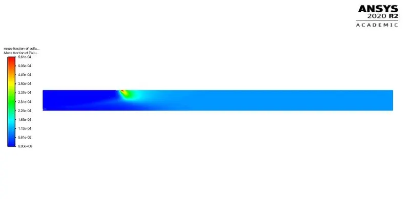
Fig. 14- Contours for mass fraction of NOx

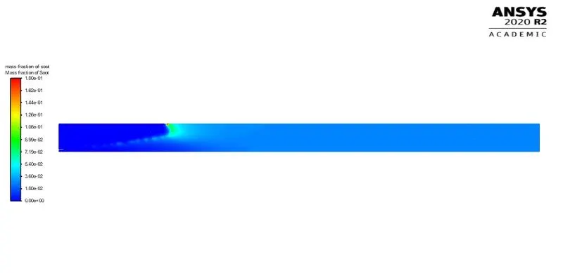
Fig. 15- Contours for mass fraction of Soot

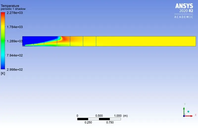
Fig. 16- Line probe drawn on PST for CH4

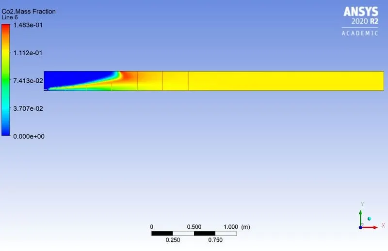
Fig. 17- Line probe drawn on PST for CO2

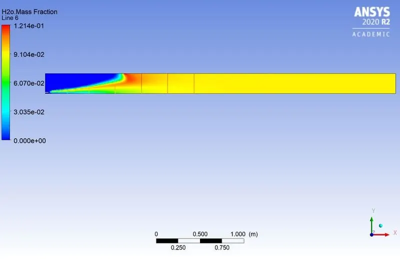
Fig. 18- Line probe drawn on PST for H2O

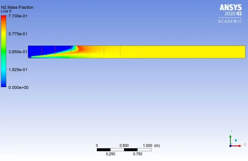
Fig. 19- Line probe drawn on PST for N2

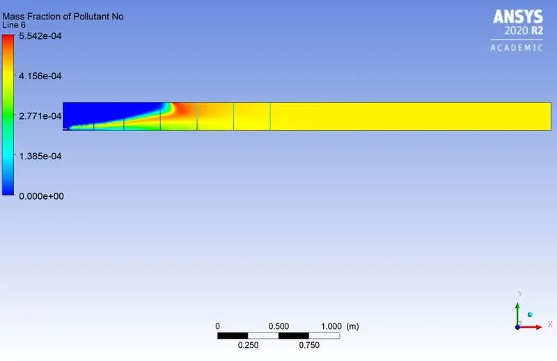
Fig. 20- Line probe drawn on PST for NOx

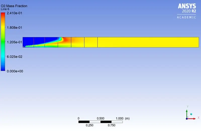
Fig. 21- Line probe drawn on PST for O2

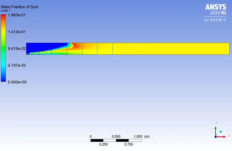
Fig. 22- Line probe drawn on PST for Soot

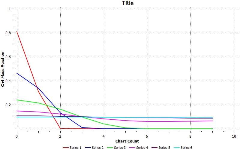
Fig.23- Chart comparission CH4

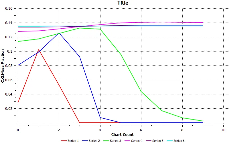
Fig. 24- Chart comparission CO2

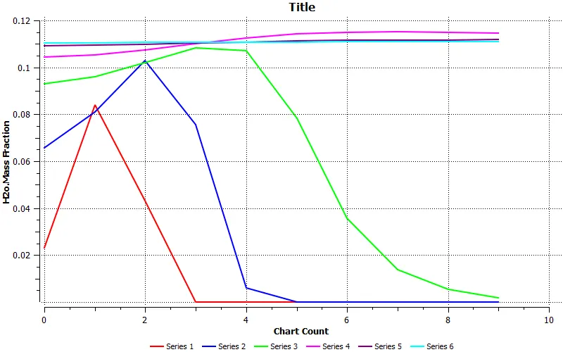
Fig. 25- Chart comparission H2O

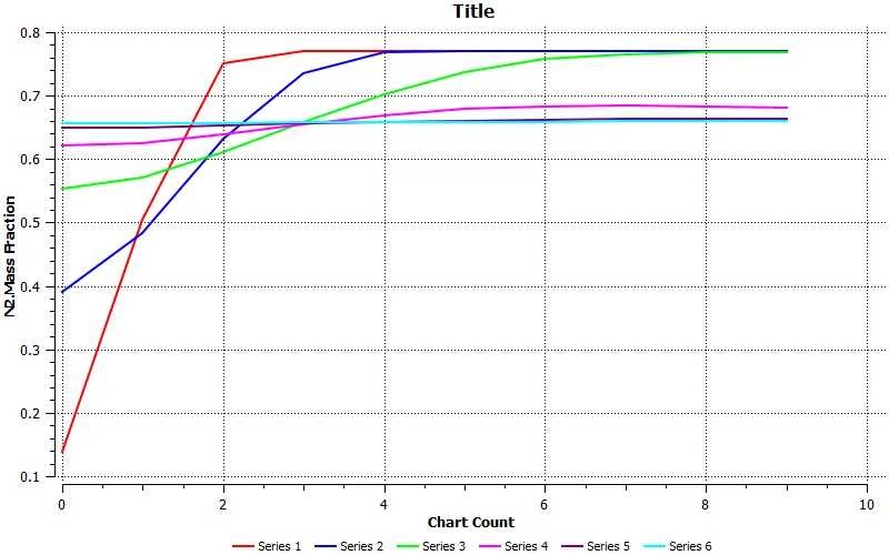
Fig. 26- Chart comparission N2

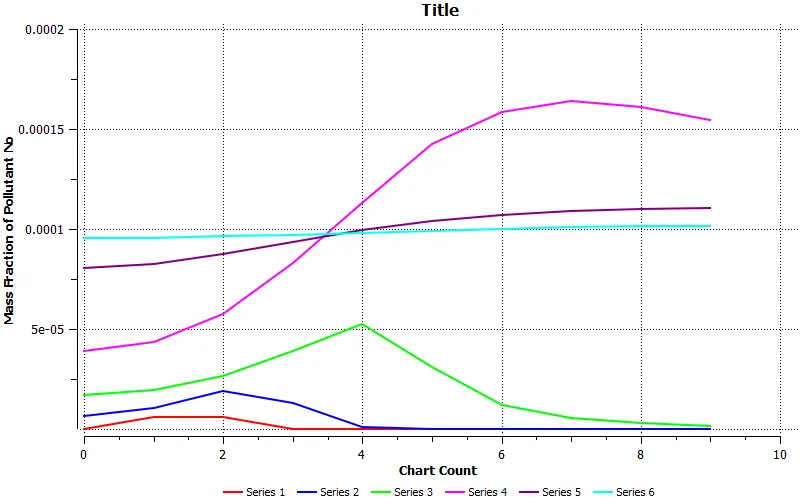
Fig.27- Chart comparission NOx

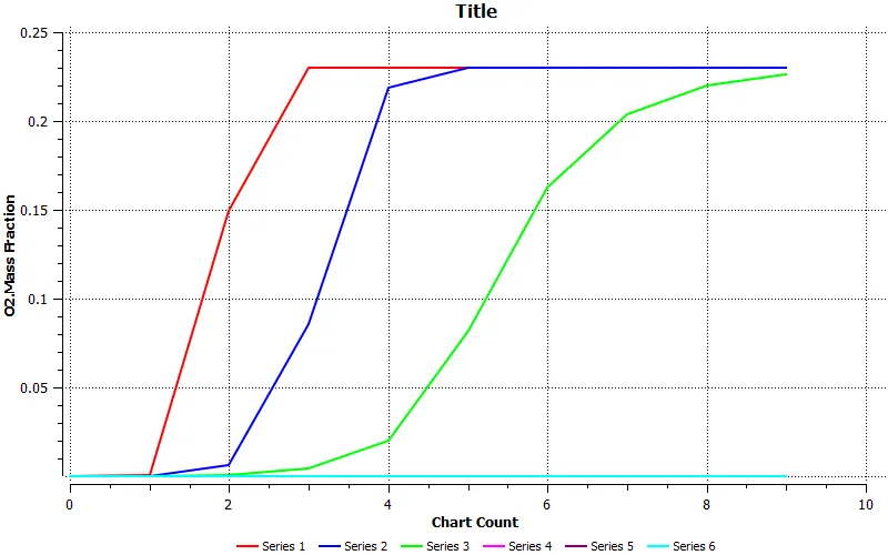
Fig. 28- Chart comparission CO2

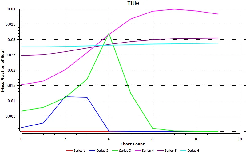
Fig. 29- Chart comparission Soot

Case II

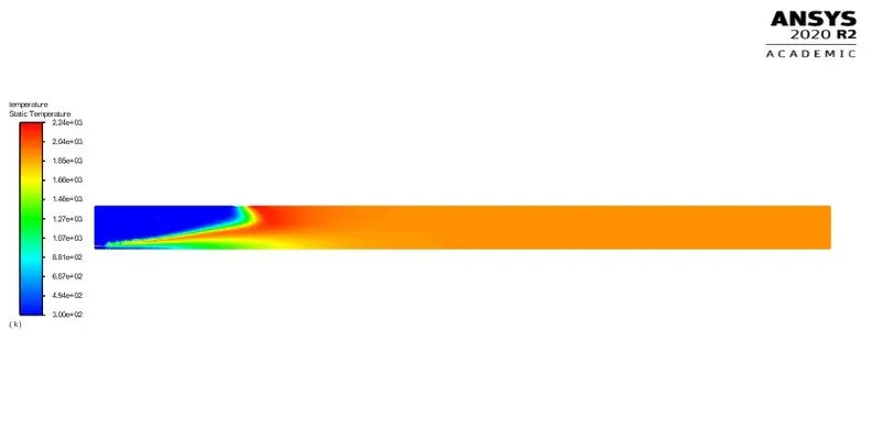
Fig. 30- Temperature contour when methane is mixed with water

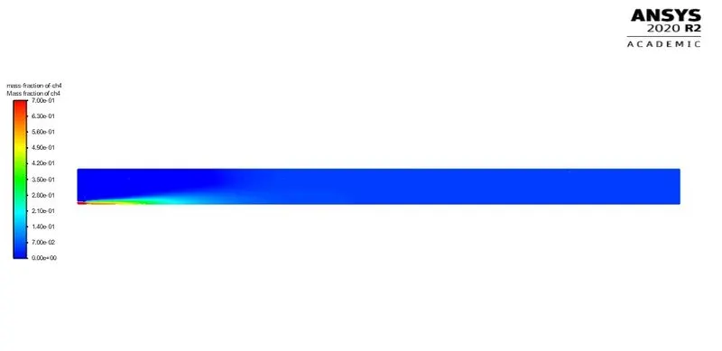
Fig. 31- Contours of mass fraction of CH4

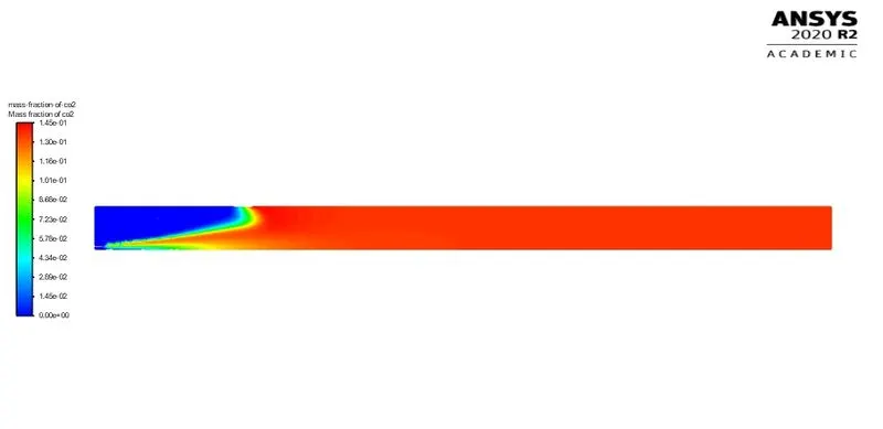
Fig. 32- Contours of mass fraction of CO2

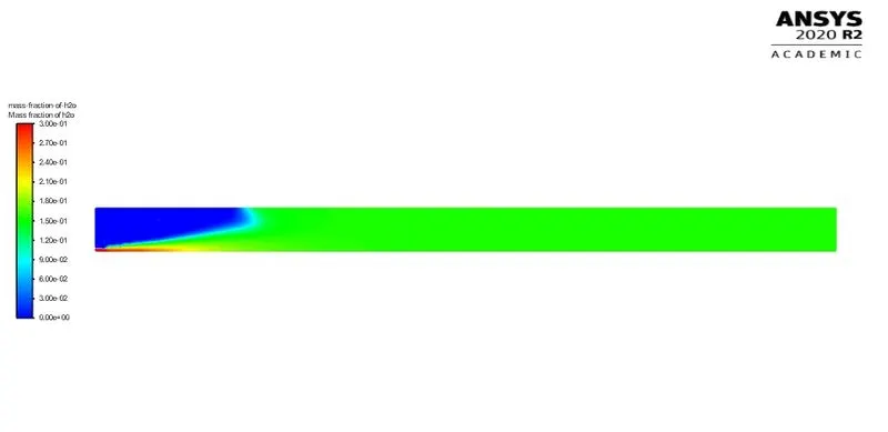
Fig. 33- Contours of mass fraction of H2O

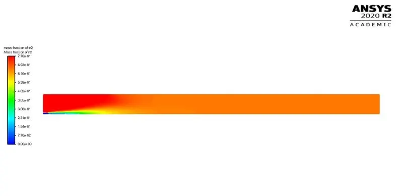
Fig. 34- Contours of mass fraction of N2

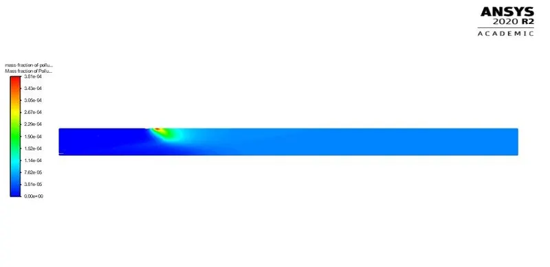
Fig. 35- Contours of mass fraction of NOx

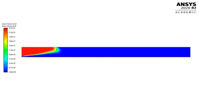
Fig. 36- Contours of mass fraction of O2

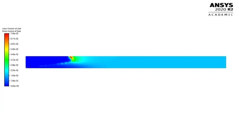
Fig. 37- Contours of mass fraction of Soot

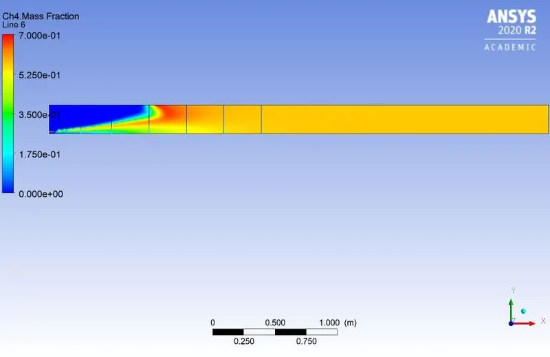
Fig. 38- Line probe drawn on PST for CH4 for case II

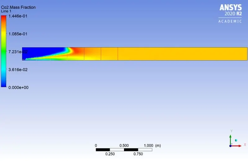
Fig. 39- Line probe drawn on PST for CO2 for case II

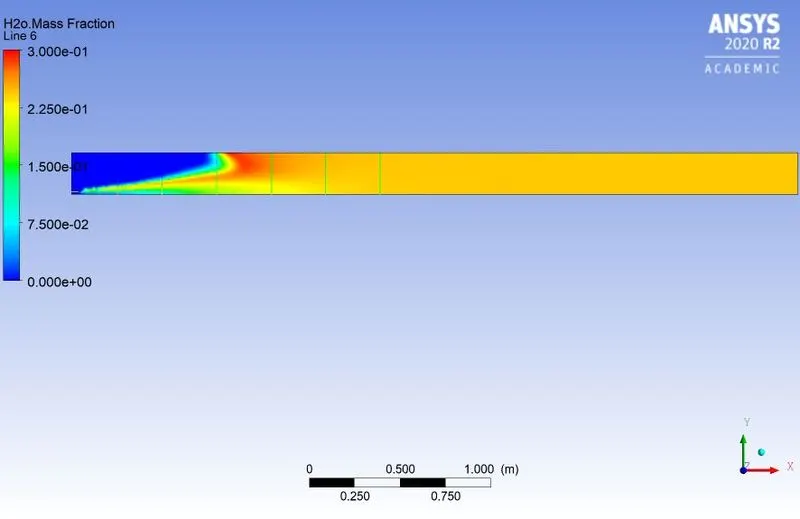
Fig. 40- Line probe drawn on PST for H20 for case II

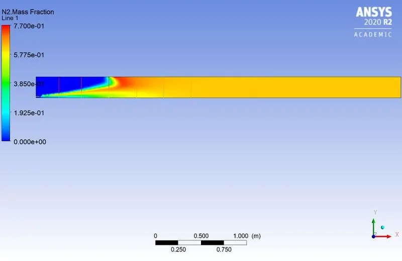
Fig. 41- Line probe drawn on PST for N2 for case II

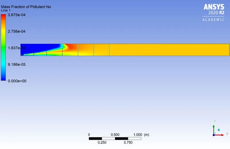
Fig. 42- Line probe drawn on PST for NOx for case II

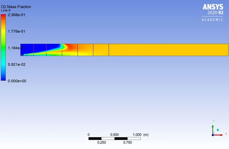
Fig. 43- Line probe drawn on PST for O2 for case II

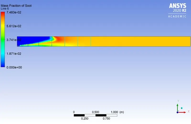
Fig. 44- Line probe drawn on PST for Soot for case II

Conclusion

Case I has a complete methane as fuel simulation where as case II has 30% by mole of methane as fuel. Observing the contours and line plots we can observe there is slight change in colour suggesting there are different rates of heat relased which implies different levels of combustion has happend. Case I the soot and NOx formation is high, but we get to use good combustion energy. Case II, when water is added in little percent also the combustion process and the results changes. The heat produced is low but the NOx and soot formation is also low. The simulation is done only taking methane as fuel and not anything else. Emissions and soot formation is makeing a huge impact on climate change which needs to be controlled. One of many ways can be the above simulation.