Week 10: Project 1 - FULL HYDRO case set up (PFI)
Project 1 - FULL HYDRO case set up (PFI)
Engine Geometric Parameters:-
- Bore =0.086 m
- Stroke = 0.09 m
- Connecting rod length = 0.18 m
- RPM = 3000
Run parameters:-
- Simulation mode: No Hydro
Simulation time parameters:-
- Start time : -520 deg
- end time : 120 deg
Boundary conditions:-
- Piston temperature - 450K
- Liner temperature - 450K
- Head temperature - 450K
- Spark Plug temperature - 550K
- Spark Plug electrode temperature - 600K
- Exhaust ports temperature - 500K
- Exhaut outflow - 1 bar
- Exhaust outlflow temperature - 800k
- Exhaust species concentration - Calculate the stoichiometric condition
- Exhaust valve top temperature - 525K
- Exhaust valve angle temperature - 525K
- Exhaust valve bottom temeprature - 525K
- Intake port - 1 temperature 425K
- Intake port - 2 temperature 425K
- Inflow pressure - 1 bar total pressure
- Inflow temperature - 363K
- Inflow species - Air
- Intake valve top temperature - 480K
- Intake valve angle temperature - 480K
- Intake valve bottom temeprature - 480K
Initial conditions:-
- Intake port - 1 (closer to combustion chamber)
- ic8h18 - 0.025508
- o2 - 0.20157
- n2 - 0.77292
- Temperature - 390k
- pressure - 1 bar
- Intake port - 2 (away from combustion chamber)
- Air
- Temperature - 370K
- Pressure - 1 bar
- Cylinder
- Pressure - 1.85731 bar
- Temperature - 1360K
- Stoichiometric composition
Injection Parameters:-
- Fuel flow rate = 7.5e-4 Kg/second
- Injection start time = -480.0
- Injection duration = 191.2
- Fuel temperature = 330K
Nozzle positions:-
Nozzle diameter = 250 micro-meter
Circular injection radius = Nozzle radius
Spray cone angle = 10
- Nozzle 0
- center 0.0823357 0.00100001 0.07019
- Align Vector -0.732501 0.210489 -0.647408
- Nozzle 1
- center 0.0823357 -0.00099999 0.07019
- Align Vector -0.732501 -0.210489 -0.647408
- Nozzle 2
- center 0.0823357 -0.0004 0.07019
- Align Vector -0.5 -0.2 -0.647408
- Nozzle 3
- center 0.0823357 0.0003 0.07019
- Align Vector -0.5 0.2 -0.647408
Spark Ignition Parameters:-
- Start of spark = -15 deg
- Spark duration = 10 deg
- Spark location = -0.003 0 0.0091
- Spark radius = 0.0005m
Aim :-
To set up a combustion simulation with the details given in the challenge and to study different properties of combustion by post processing the results obtained by the calculation of the full hydrodynamic set up of the given geometry.
Objective :-
1. What is the compression ratio of this engine?
2. Why do we need a wall heat transfer model? Why can't we predict the wall temperature from the CFD simulation?
3. Calculate the combustion efficiency of this engine
4. use the engine performance calculator, to determine the power and torque for this engine.
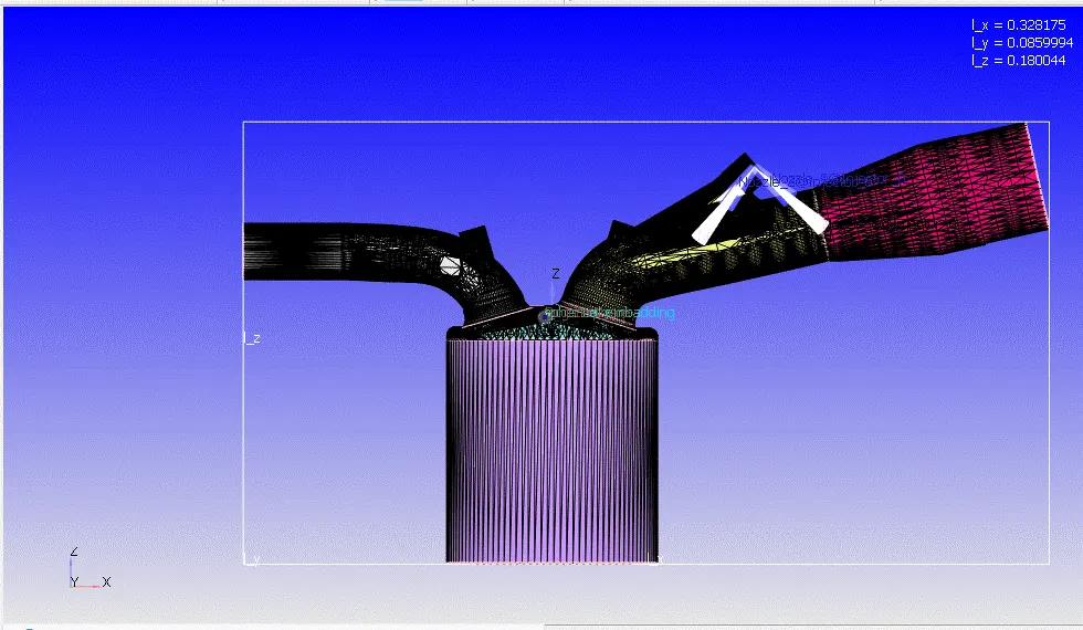
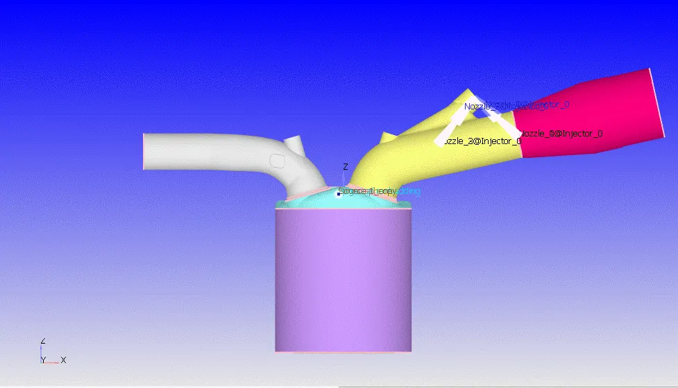
Geometry :-
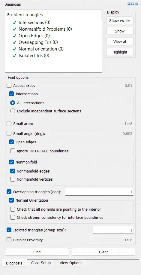
Diagnosis :-
Case Setup :-
The application type is set to Crank angle based as we are simulating an IC engine cylinder.
The measurements for the cylinder are specified by refering to the given data file.
Cylinder Bore : 0.086 m
Stroke : 0.09 m
Connecting rod length : 0.18 m
Crank speed : 3000 RPM
Specify the reference boundaries as given below, so that the motion of the simulations takes place at the right boundaries.
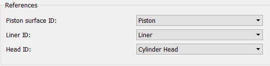
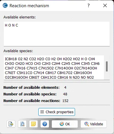
Import the mech.dat and therm.dat in the materials tree to specify the reactions taking place between the materials inside the cylinder during combustion.
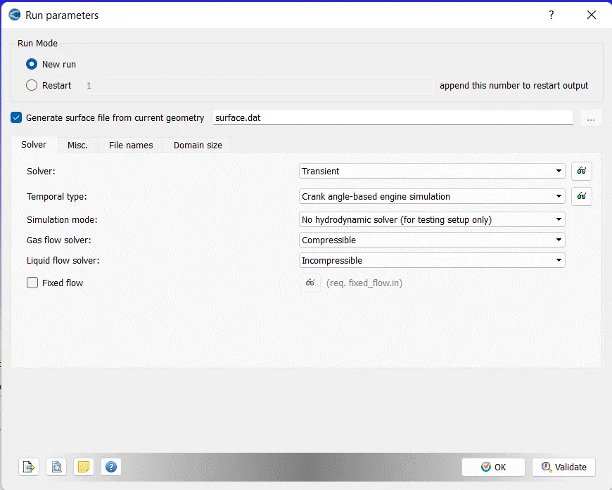
In the run parameters, set up a transient simulation and select No Hydrodynamic solver as simulation mode. The gas flow solver is set to be compressible.
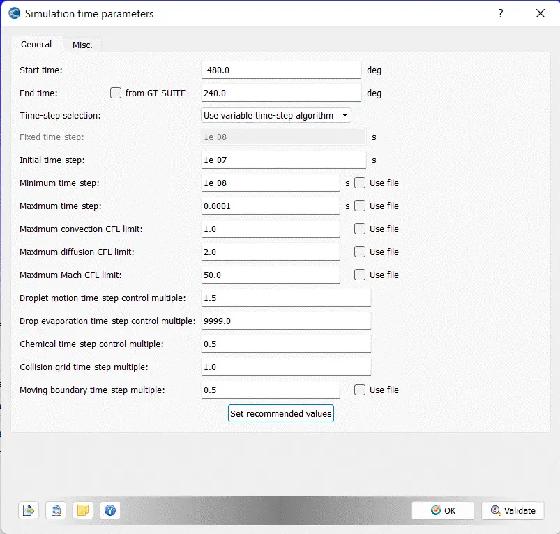
The simulation time parameter is set from -480 degree to 240 degree as the simulation is made to run for a total of 720 degree angle.
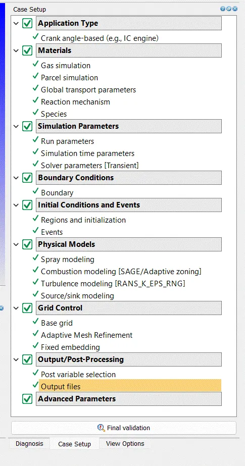
Crank Angle- Based :-
- Bore =0.086 m
- Stroke = 0.09 m
- Connecting rod length = 0.18 m
- RPM = 3000
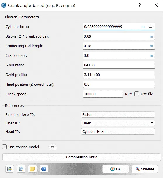
Case Setup :-
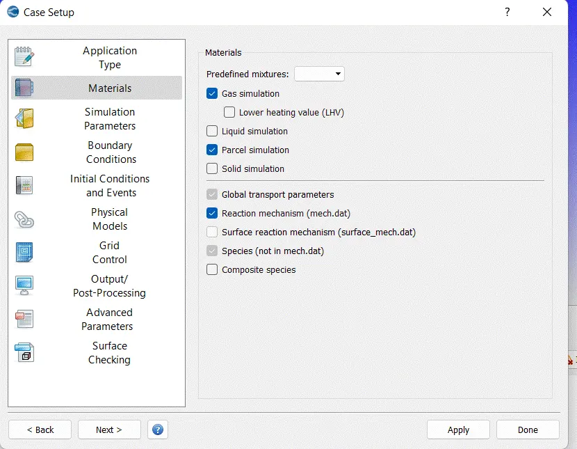
Gas Simulation :-
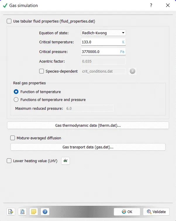
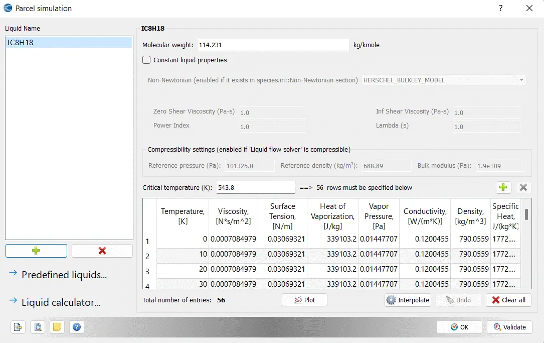
Parcel Simulation :-
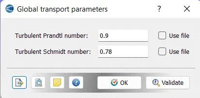
Global Transport Parameters :-
Reaction Mechanism :-
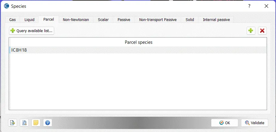
Species :-
Run Parameters :-
Run parameters:-
- Simulation mode: No Hydro
Simulation Time Parameters :-
Solver Parameters[Transient] :-
Boundary :-
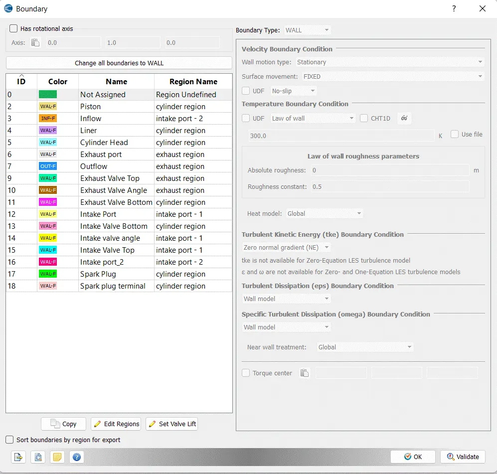
Boundary conditions:-
- Piston temperature - 450K
- Liner temperature - 450K
- Head temperature - 450K
- Spark Plug temperature - 550K
- Spark Plug electrode temperature - 600K
- Exhaust ports temperature - 500K
- Exhaut outflow - 1 bar
- Exhaust outlflow temperature - 800k
- Exhaust species concentration - Calculate the stoichiometric condition
- Exhaust valve top temperature - 525K
- Exhaust valve angle temperature - 525K
- Exhaust valve bottom temeprature - 525K
- Intake port - 1 temperature 425K
- Intake port - 2 temperature 425K
- Inflow pressure - 1 bar total pressure
- Inflow temperature - 363K
- Inflow species - Air
- Intake valve top temperature - 480K
- Intake valve angle temperature - 480K
- Intake valve bottom temeprature - 480K
Regions And Initialization :-
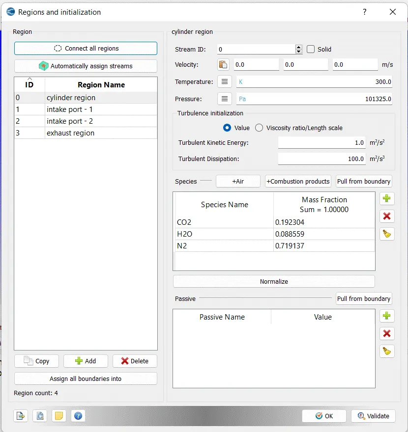
Initial conditions
- Intake port - 1 (closer to combustion chamber)
- ic8h18 - 0.025508
- o2 - 0.20157
- n2 - 0.77292
- Temperature - 390k
- pressure - 1 bar
- Intake port - 2 (away from combustion chamber)
- Air
- Temperature - 370K
- Pressure - 1 bar
- Cylinder
- Pressure - 1.85731 bar
- Temperature - 1360K
- Stoichiometric composition
Events :-
Spray Modeling :-
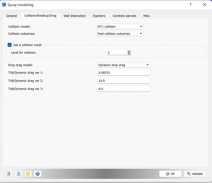
Collision/Breakup/Drag :-
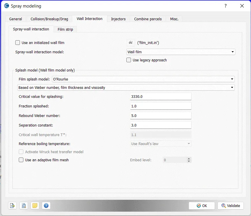
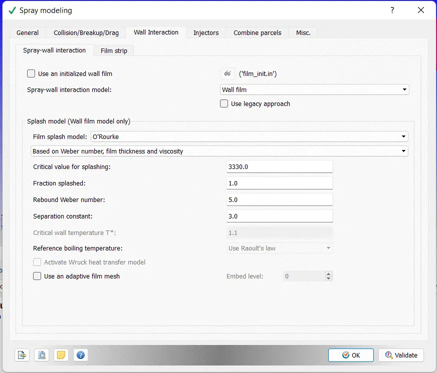
Wall Interaction :-
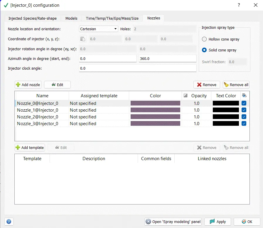
Injectors :-
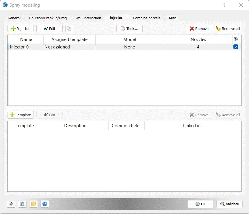
Injectors :-
injected species/rate-shape
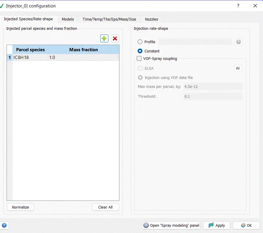
Injectors :-
Models
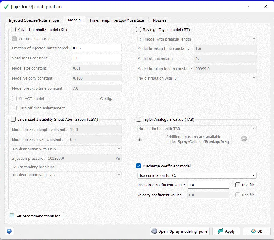
Injectors :-
Time/Temp/Tke/Eps/Mass/Size
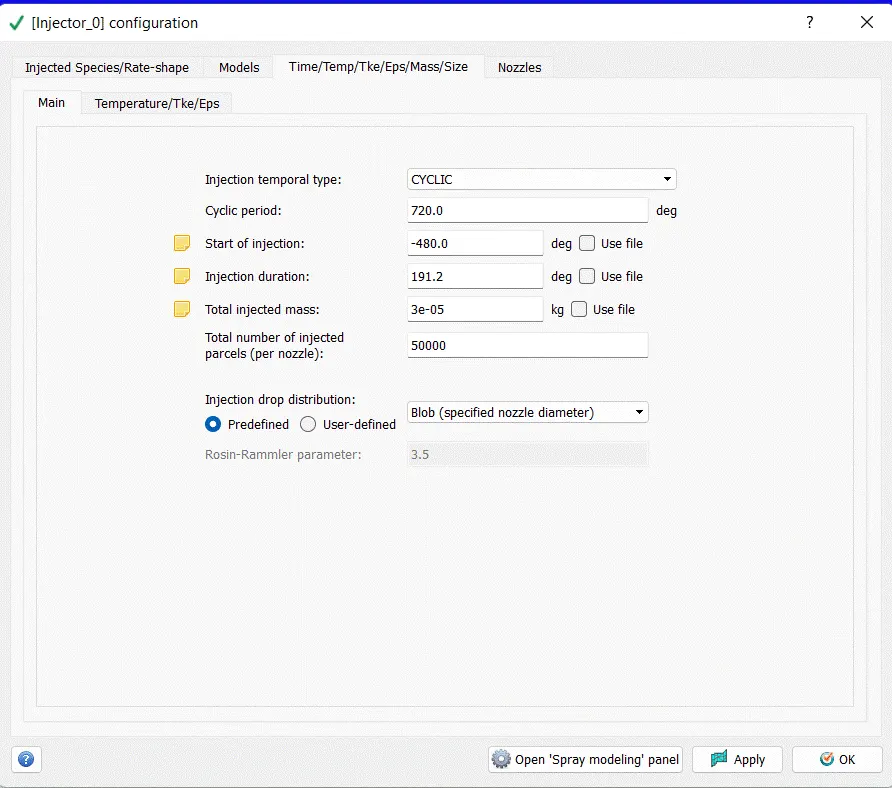
Injectors :-
Nozzles
Nozzle positions:-
Nozzle diameter = 250 micro-meter
Circular injection radius = Nozzle radius
Spray cone angle = 10
- Nozzle 0
- center 0.0823357 0.00100001 0.07019
- Align Vector -0.732501 0.210489 -0.647408
- Nozzle 1
- center 0.0823357 -0.00099999 0.07019
- Align Vector -0.732501 -0.210489 -0.647408
- Nozzle 2
- center 0.0823357 -0.0004 0.07019
- Align Vector -0.5 -0.2 -0.647408
- Nozzle 3
- center 0.0823357 0.0003 0.07019
- Align Vector -0.5 0.2 -0.647408
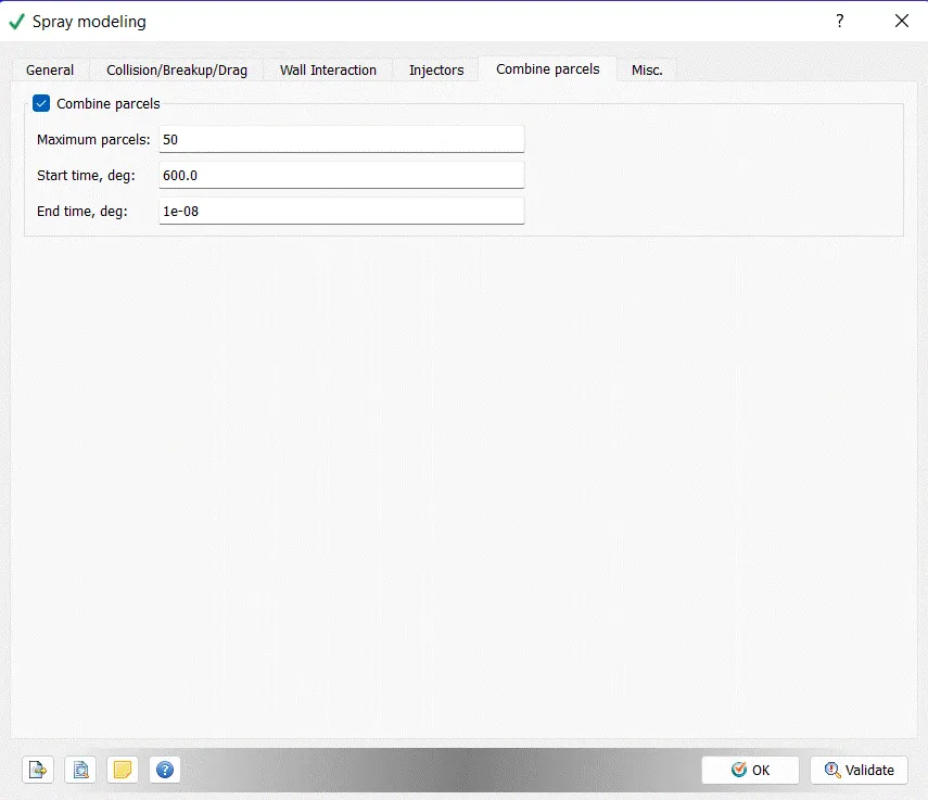
Combine Parcels :-
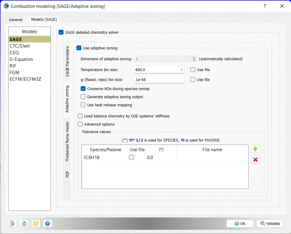
CONVERGE’s SAGE detailed chemistry solver uses local conditions to calculate reaction rates based on the principles of chemical kinetics. This solver is fully coupled to the flow solver, but the chemistry and the flow solvers parallelize independently of one another, which speeds up the simulation. With the appropriate mechanism, the SAGE solver can predict a wide range of cases (e.g., a variety of fuels [premixed, non-premixed, partially premixed, multiple fuels], emissions modeling, and unique phenomena such as end-gas auto-ignition). With its accuracy and robustness, CONVERGE can perform predictive modeling instead of merely confirming experimental results.
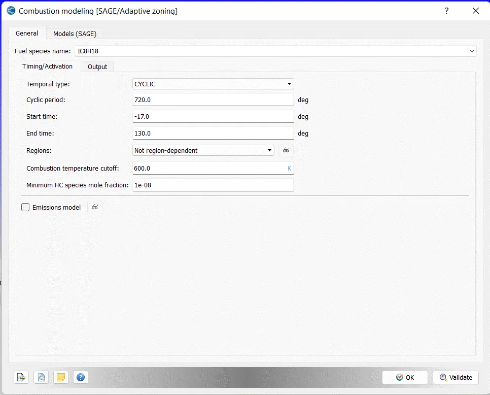
The next step in the modeling is the combustion modeling parameter. The values for the combustion properties like start time, end time & species is to be specified as given in the image below.
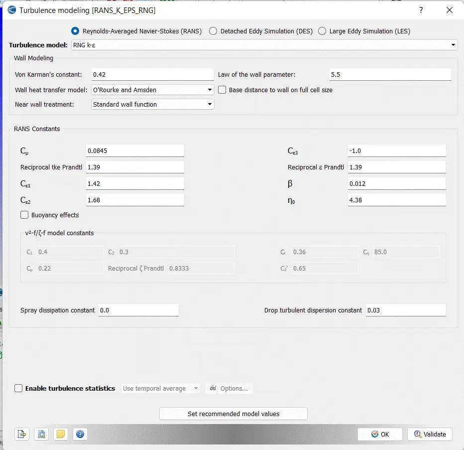
The combustion model here is taken as the SAGE model. The turbulence model is taken as the RNG K-Eppsilon model.
Combustion Modeling[SAGE/Adaptive zoning] :-
General
Models(SAGE) :-
Turbulences Modeling [RANS_K_EPS_RNG] :-
Source/Sink Modeling :-
Then the source of power should be specified in order to ignite the incoming fuel during the compression of the fuel. For this select source modeling under the physics modeling.
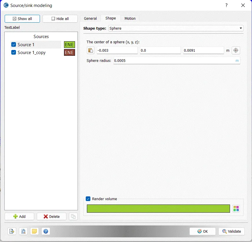
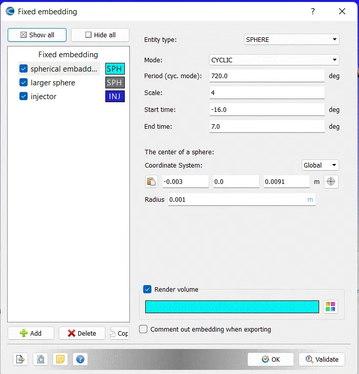
In the source modeling add two sources where both the sources have a spherical shape.
Spark location = -0.003 0 0.0091
Spark radius = 0.0005m
The spark location and radius specifies the spherical volume where the ignite starts.
The time interval for the spark is given in degree.
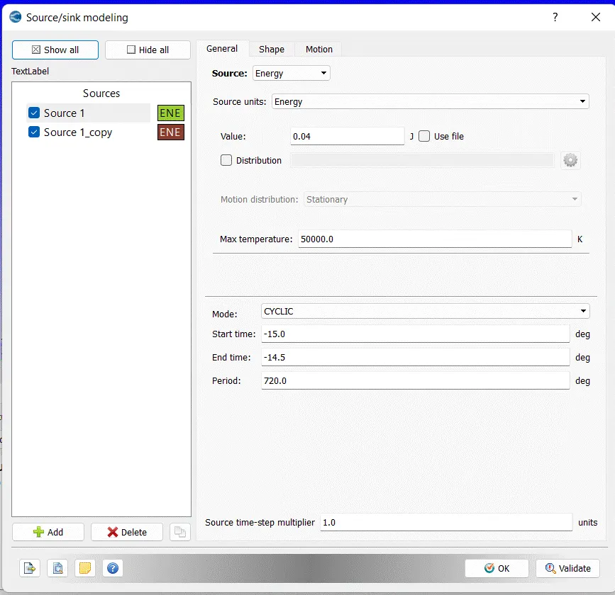
Source/Sink Modeling :-
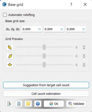
Base Grid :-
The grid size is taken to be 0.004 m and fixed embeddings are done at critical points.
The valve angles are provided with a scaling of 3 as they are moving so close to the walls of the cylinder head.
The mesh inside the cylinder is also refined to a scale of 2 as the combustion can be captured properely.
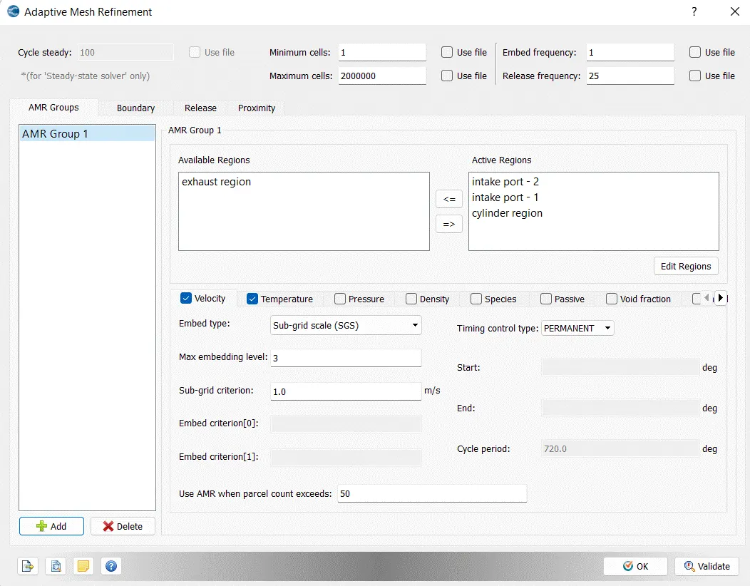
AMR :-
Fixed Embedding :-
To refine that critical area, we can use Fixed Embedding around the Throttle Boundary.
fixed embedding is used to refine the grid at specific locations in the domain where a finer resolution is critical to the accuracy of the solution. Fixed embedding allows the rest of the grid to remain coarse to minimize simulation time.
For each fixed embedding, you must specify an embedding scale that indicates how CONVERGE will refine the grid in that location. The embed_scale parameter, which must be a positive integer, scales the base grid sizes (dx_base, dy_base, and dz_base) according to
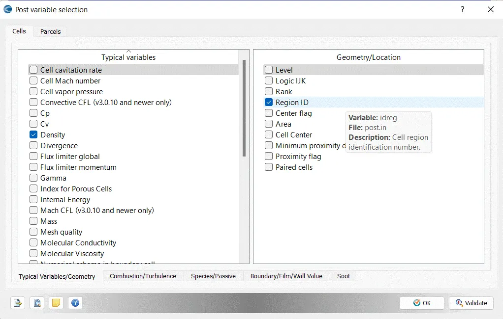
Post Variable Selection :-
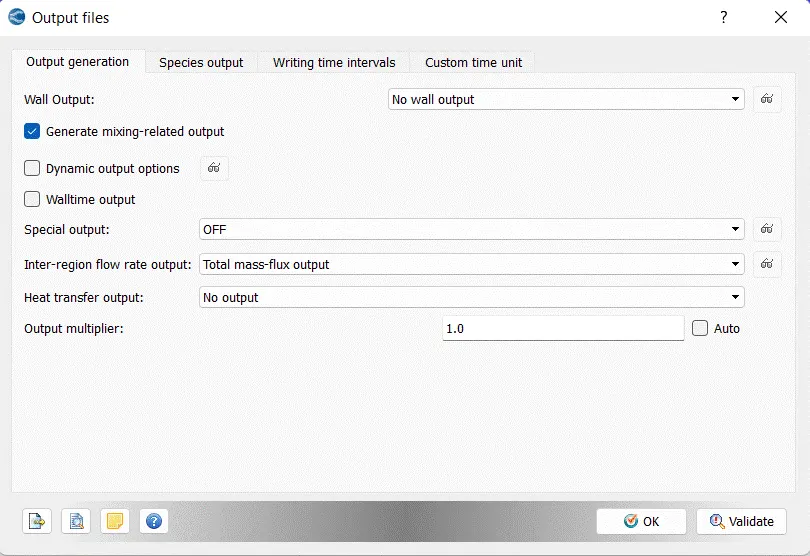
Output Files :-
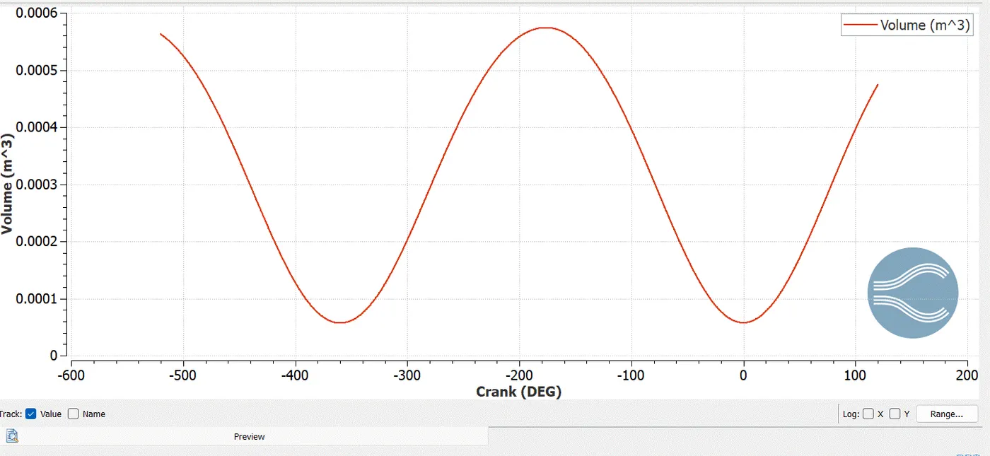
Plotting :-
Volume(m^3)
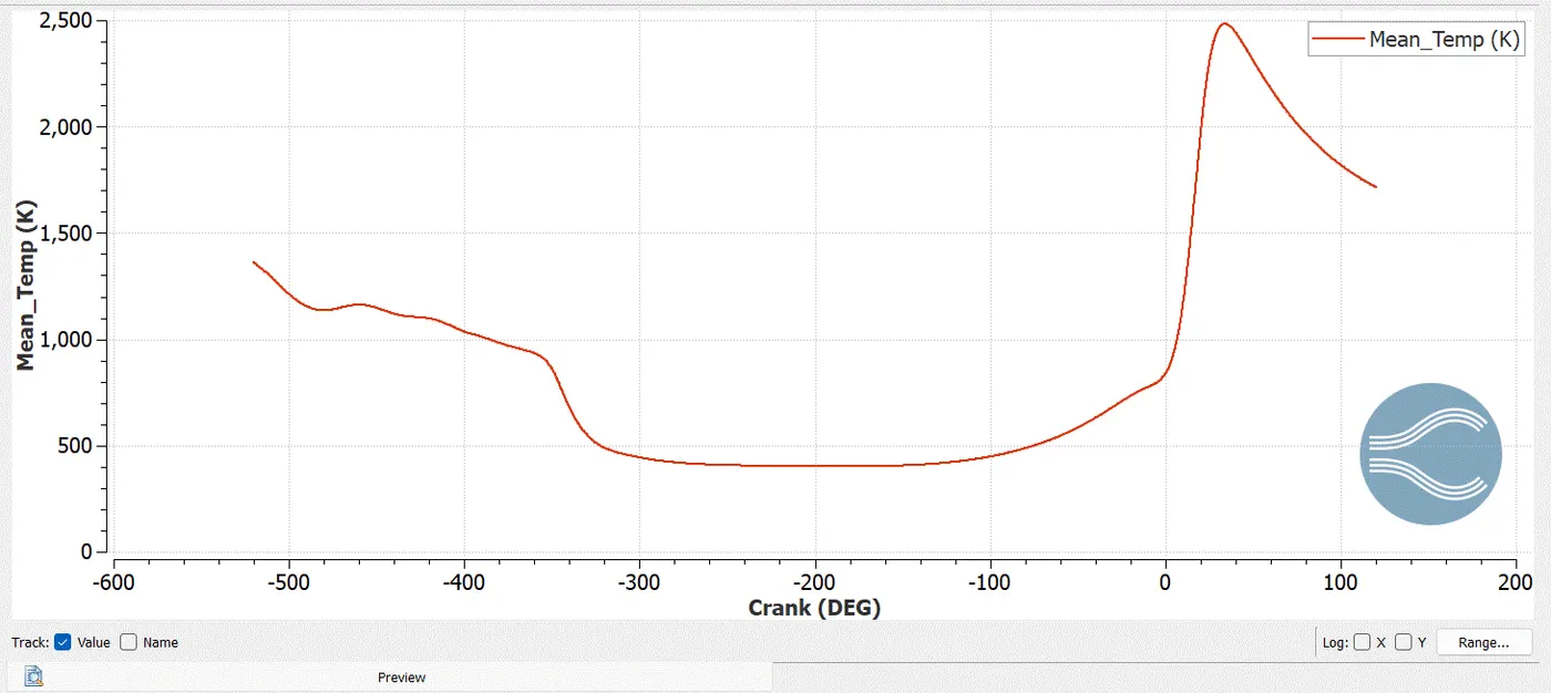
Mean_Temp(k) :-
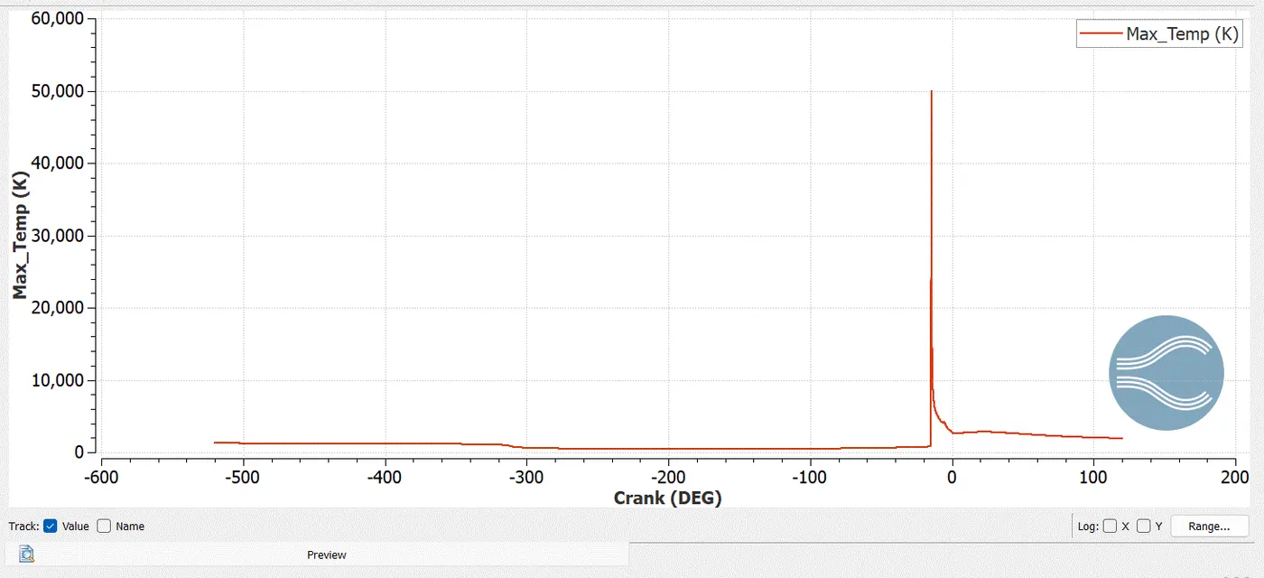
Max_Temp :-
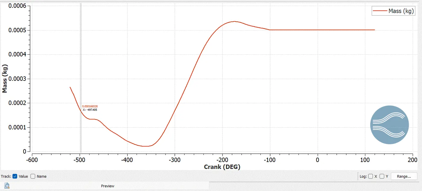
Mass(kg) :-
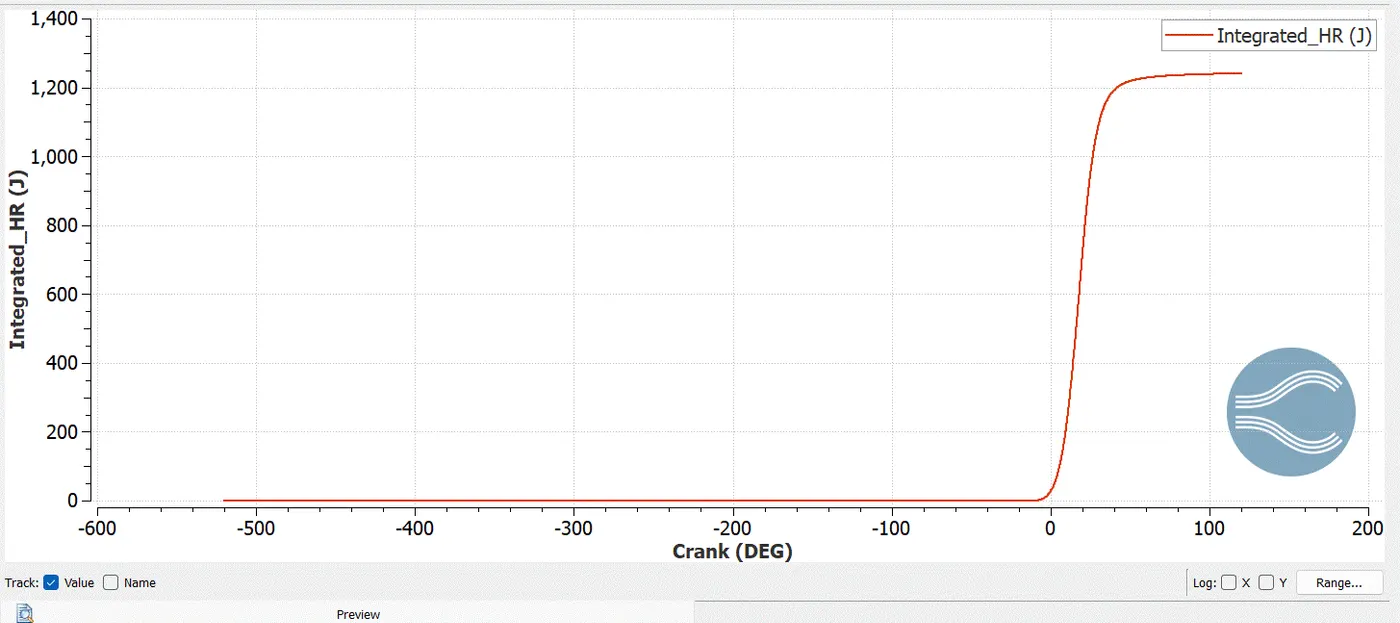
Integrated_HR(J) :-
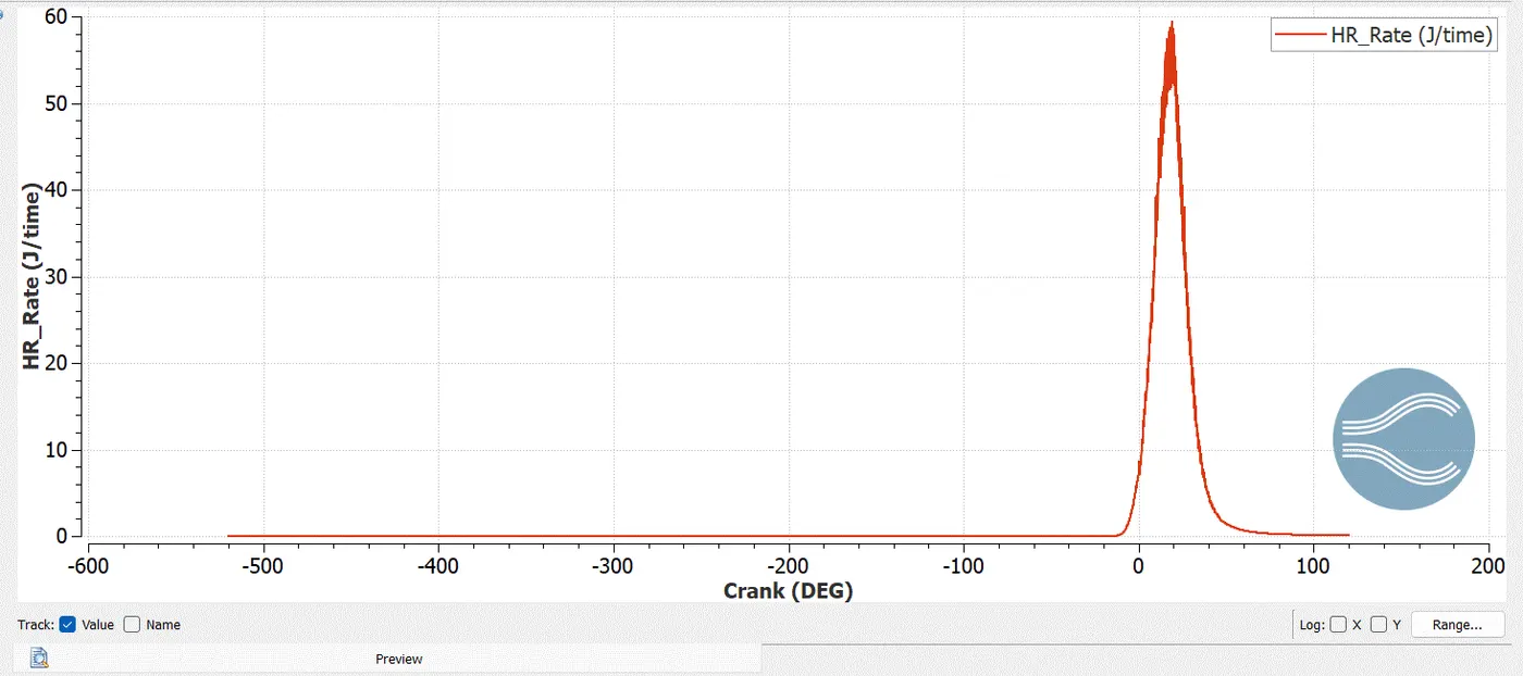
HR_Rate(j/time) :-
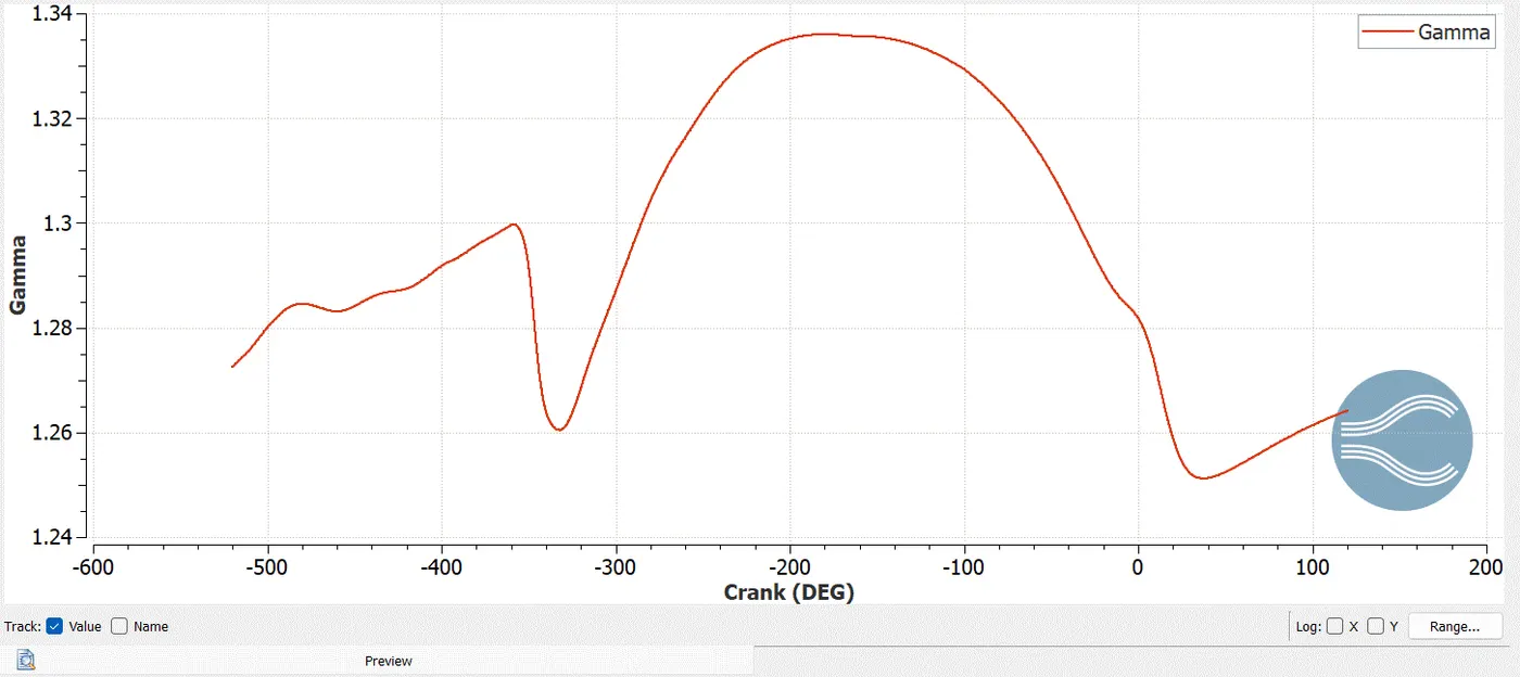
Gamma :-
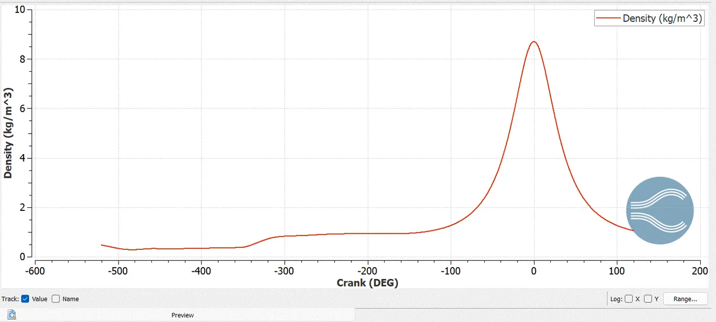
Density(kg/m^3) :-
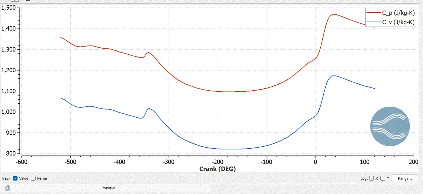
C_p (j/kg-k)
C_v (j/kg-k)
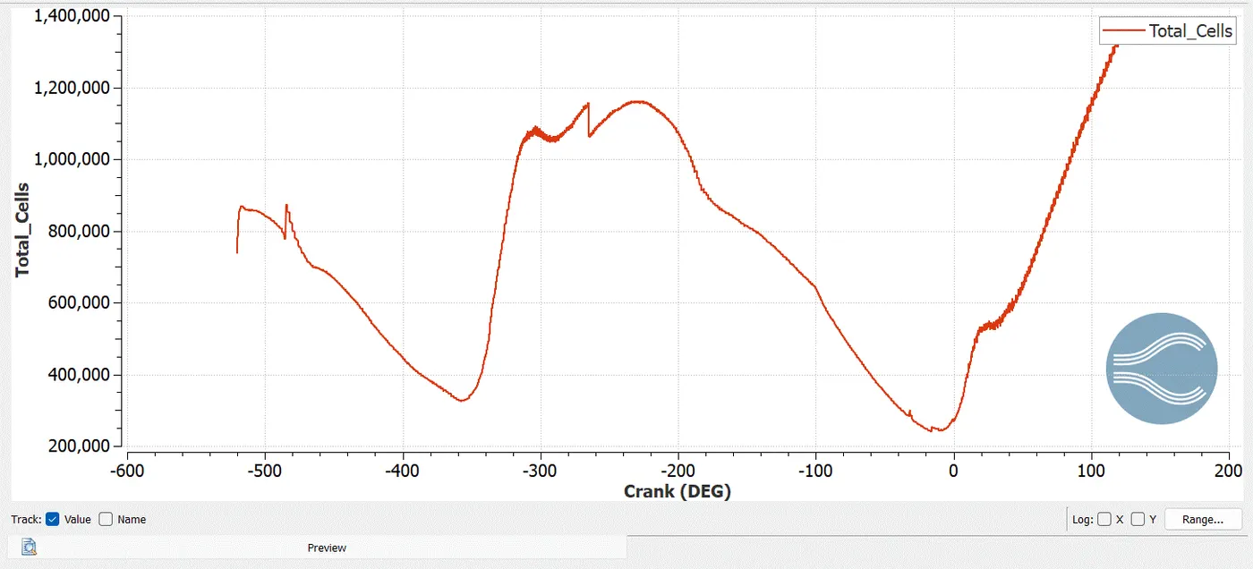
Total_cells Count :-