Week - 10 Hyperelastic Material Models

Week -10 Hyperelastic Material models

AIM

To calculate the Mooney Rivlin and Ogden material constants and compare both of the stress-strain data curves with the simulated stress-strain data of a dogbone specimen model which is subjected to tensile test with 100 percent strain.

Theory of Hyperelastic materials

Hyperelastic materials are materials that take a large amount of strain (500% strain ) and still come back to their original position when the stretch is released. They respond elastically when they are subjected to a large number of strains. The mechanical behavior of hyperelastic material is expressed in terms of the strain energy function. The strain energy function is typically a function of stretch. Ogden rubber, hyperelastic rubber are some examples of hyperelastic materials.

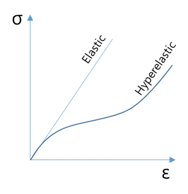
Fig, represents the stress-strain curve of hyperelastic models, indicating that hyperelastic models take a large strain and behaves elastically.

MECHANICAL TEST DATA OF HYPERELASTIC MODELS

• The mechanical test data of the hyperelastic models are obtained from the simple deformations tests such as, uniaxial tension, equibiaxial compression, uniaxial compression, equibiaxial tension, planar tension and planar compression.
• In this challenge, the mechanical test data is obtained from the uniaxial tension test.
• The mechanical test data are used to evaluate the material constants of the hyperelastic model, which is used for evaluating the behaviour of the hyperplastic model.

PURPOSE OF EVALUATING MATERIAL CONSTANTS

• The purpose of evaluating, the material constant is to get the mechanical response to the hyperelastic model.
• In order to get the correct analysis of the results, we need to evaluate the material constant.
• The material constants can be evaluated by inputting the stress-strain data to LS-DYNA software.

STRAIN ENERGY FUNCTION FOR BOTH HYPERELASTIC MODELS

Mooney Rivlin

The strain energy density function for an incompressible Mooney–Rivlin material is defined as

Where `Cij`are empirically determined material constants, `I1`and `I2` are the first and the second invariant. By varying the Index values of `i` and `j` we can change the constitutive equations and use it appropriately for our component. Similarly, we will be having multiple coefficients C. This changing of the index will be basically changing the order of the polynomial of the energy density equation

We need to find out the coefficients of these material models for a different order of the polynomial and extract the best fit curve data from the D3HSp file and compare it with the material curve.

*MAT_077_o *MAT_OGDEN_RUBBER

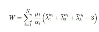
Ogden Hyper-elastic model is the expressed the strain energy function W in terms of principal stretches `λ1`, `λ2`, and `λ3` Where N is the order of the model, usually, N takes a number between 1–8. `µ_i` and `α_1` are material constants, where the unit of `µ_i` is pressure, `α_1` is a dimensionless quantity.

PROCEDURE FOR MODELLING HYPERELASTIC MATERIAL

• Initially, the image containing engineering stress and engineering strain data is downloaded and exported to MS-EXCEL.
• As we are modelling the hyperelastic material we need to define the hyperelastic materials with the stress-strain data and with the material properties.

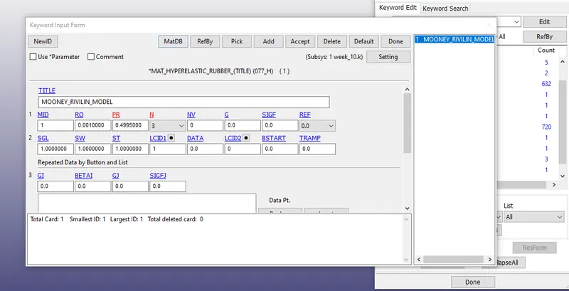
Fig, represents the material properties defined for the hyperelastic rubber

• In a similar fashion, the material properties and the load curve for Ogden rubber are defined.

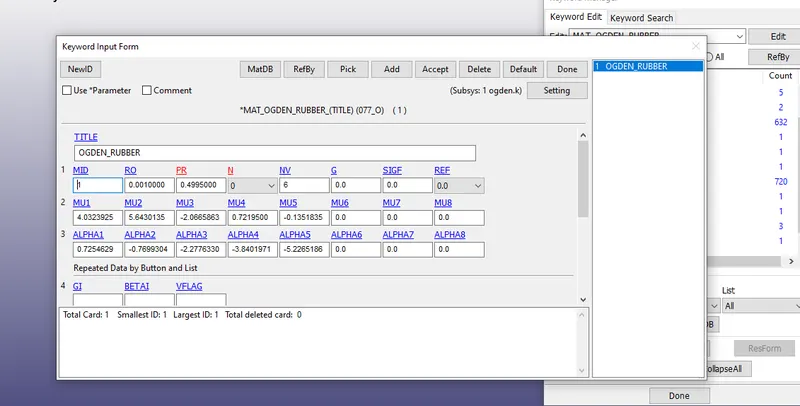
Fig, represents the material properties defined for the Ogden rubber

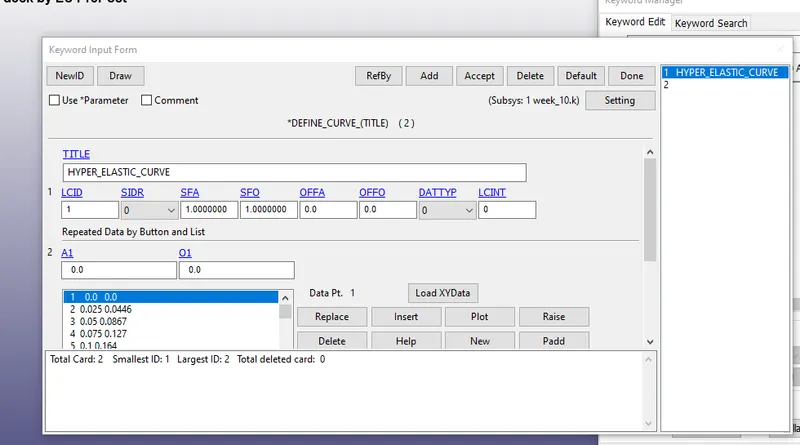
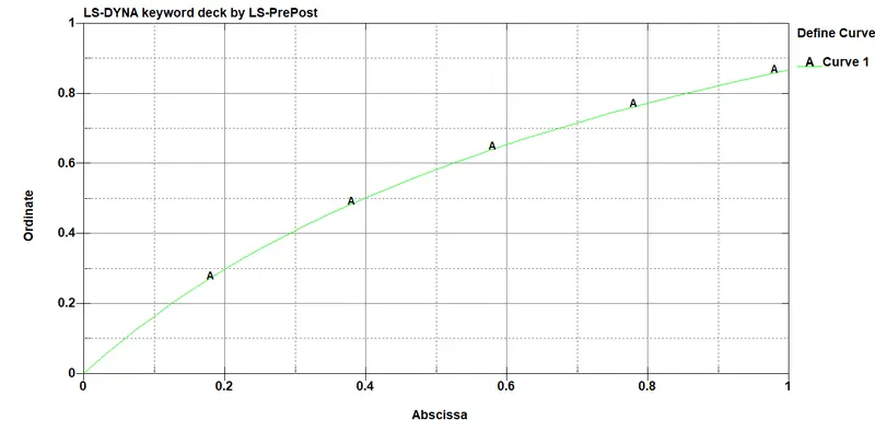
• The stress-strain which has engineering stress and strain has been inputted into to the *Define_ curve card with LCID
• The procedure is the same for Ogden rubber.

PROCEDURE FOR TENSILE TESTING

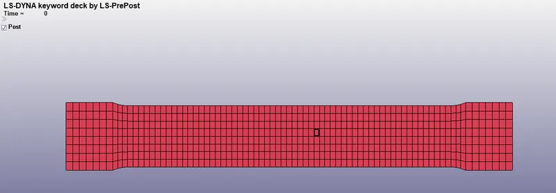
• The given dog bone specimen is opened in the LS-PRE POST.

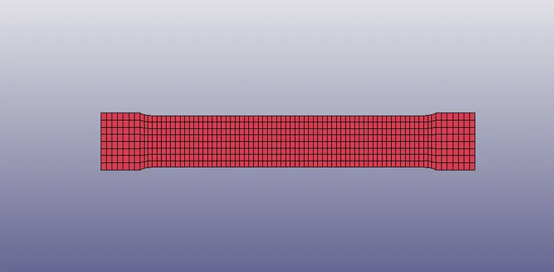
Fig, represents the dog bone specimen in LS -DYNA

• once, everything is done, now apply boundary conditions to the dog bone specimen.
• Now, for conducting the tensile test, the dog bone specimens is fixed at the one end and its y (lateral) nodes constrained are allowed to freely at the top and at the bottom and while the middle nodes are fixed.

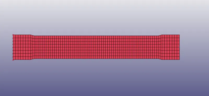
Figure, represents the nodes that are constrained in the (Y) one end and at the middle at both ends .

• The nodes are allowed to move freely, in the lateral direction when the displacement is applied.

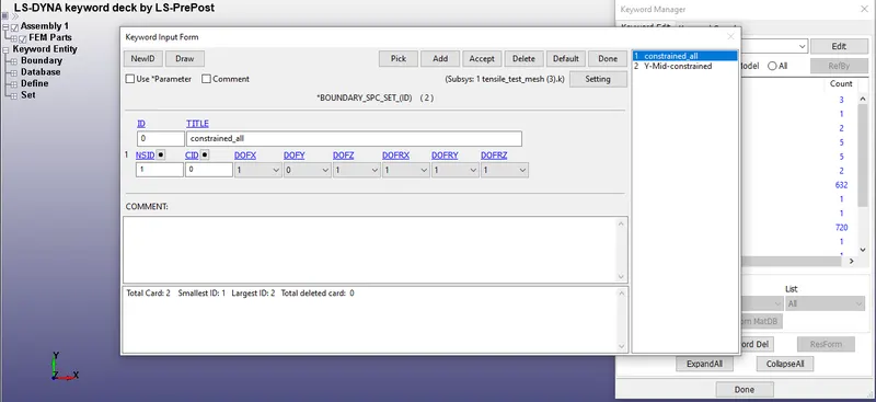
Fig,represents the nodes that are allowed to move freely in the Y-direction.

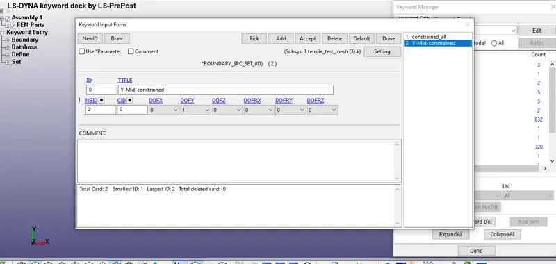
Fig, represents the Middle Y constrain of the nodes at the both the ends.

• In the section, the section shell is selected with the element formulation 2.

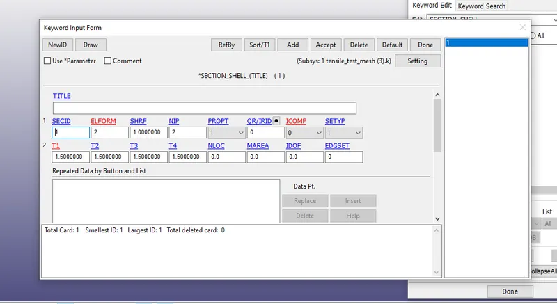
Fig, represents the section shell is defined.

• After, assigning the section, go to the part and assign the material and sec ID to the part.
• Before, giving the initial displacement now we need to calculate the stretch.
• Here we take, the displacement value of 1 since we have 100% engineering strain.
  

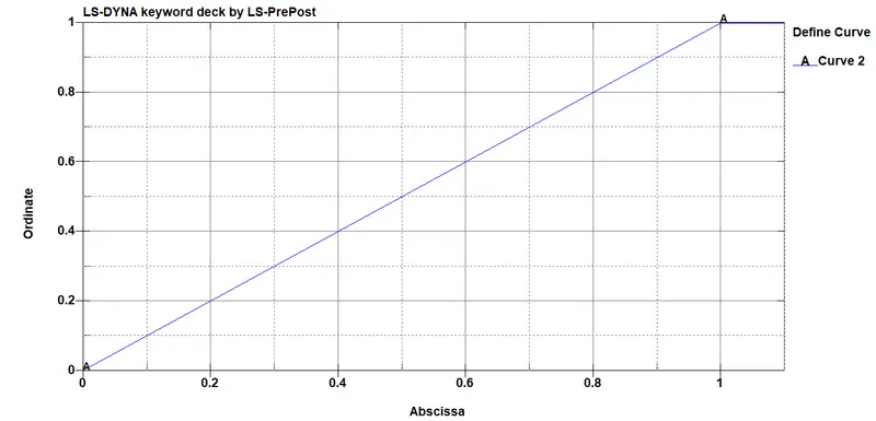
Fig, represents the displacement defined in the define curve option.

• once ,everything is done now we need to define the terimination time in the problem .

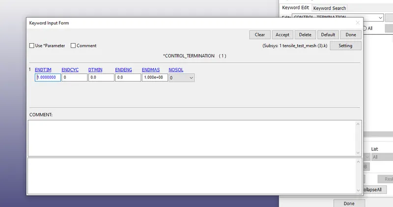
Fig, represents the termination time defined in the control termination card.

• once, everything is done we need to activate the implicit analysis for solving the problem.
• For that, we need to activate the implicit auto card for optimizing the number of iterations for solving the problem in a small interval.

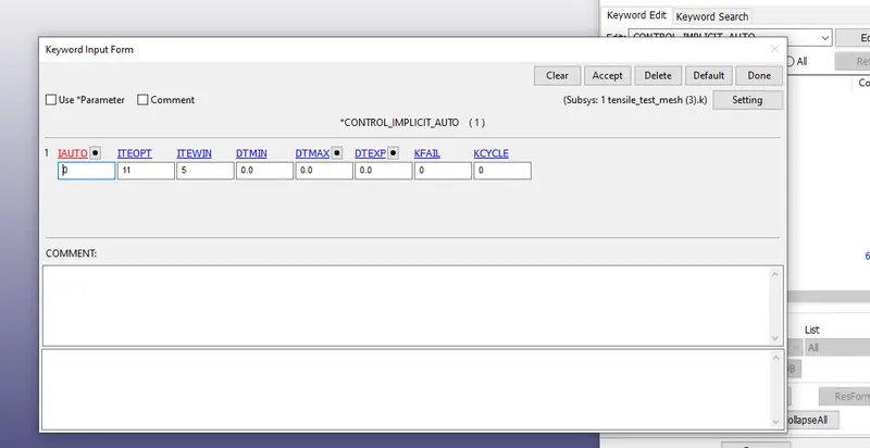
Fig, represents the ITEOPT and ITEWIN defined in the control implicit card.

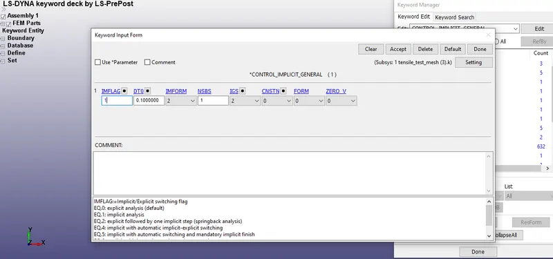
Fig, represents the activation of IMFLAG and assignment of dt in the control implicit general.

• Then, activate other implicit cards such as implicit general and implicit solver for solving the non-linear problem.

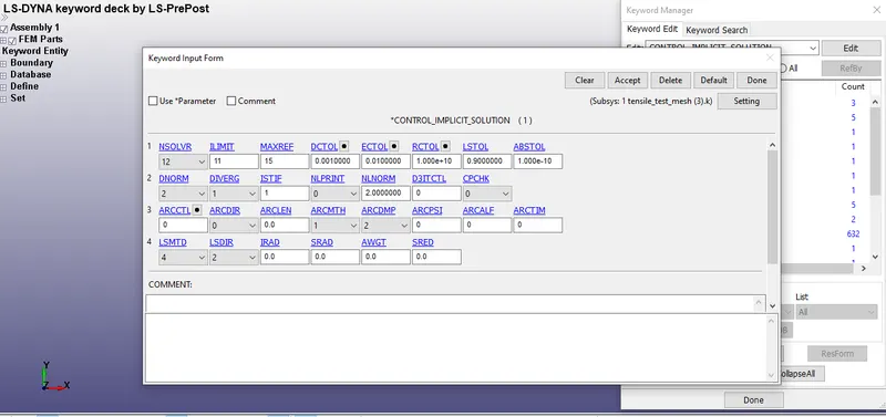
Fig, represents the activation of the control implicit solution card.

• Here, we activate the Nsolver (12) for activating the non-linear analysis.

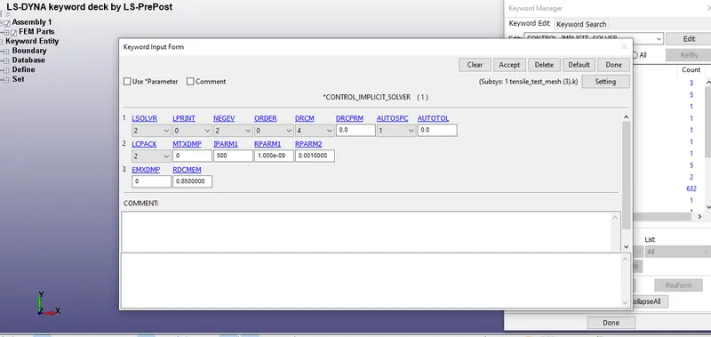
Fig, represents the activation of control implicit solver.

• Here, we activate the control implicit solver to solve or run the non-linear problem.
• Finally, we need to define the required output in the ASCII option.

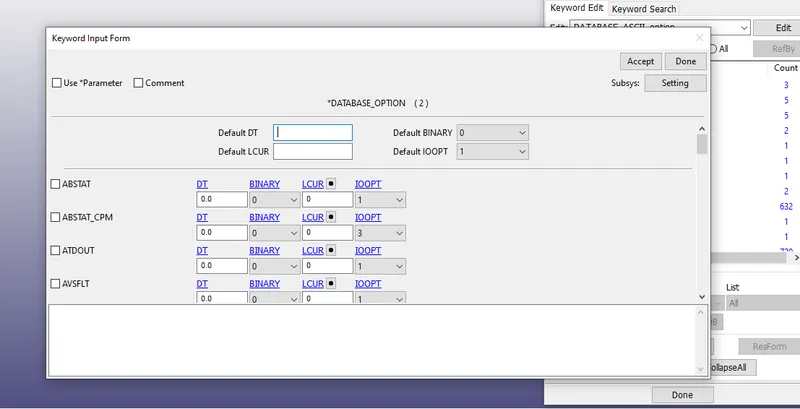
Fig, represents the assignment of GLSTAT and ELOUT in the ASCII option.

• The outputs are defined with the interval of 0.01
• Then, the output is defined with the binary d3 plot option.

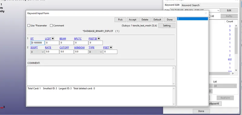
Fig, represents the defining of the database binary D3 plot.

• Here, we define the output with the dt interval of 0.1 for getting the output.
• Finally, the problem is solved using LS - Run and we got the normal termination of the mode.
• The tensile testing procedure is the same for the Ogden model.

OUTPUT RESULTS

EXTRACTING MATERIAL CONSTANT AND FIT CURVE DATA FOR EACH ORDER OF POLYNOMIAL FROM D3hsp file

• The Mooney-Rivlin constants for each case are stored in the d3hsp file

For first-order polynomial N=1 ,

Mooney constant C01 = 0.1768E+00

Mooney constant C10 = 0.1474E+00

Final Fit Data from the d3hsp file is generally in Stretch vs True Stress but We have to Covert them into Engineering Strain vs Engineering Stress

Engineering Strain = Stretch -1

Engineering Stress = True Stress/(1+Engineering strain)

For first-order polynomial N=2 ,

Hyperelastic Constant C10= 0.2595E+00

Hyperelastic Constant C01= 0.4594E-01

Hyperelastic Constant C11= -0.2092E-01

Hyperelastic Constant C20= 0.2914E-02

Hyperelastic Constant C02= 0.1016E-02

Hyperelastic Constant C30= 0.0000E+00

For first-order polynomial N=3,

Hyperelastic Constant C10= 0.2611E+00

Hyperelastic Constant C01= 0.4420E-01

Hyperelastic Constant C11= -0.6074E-02

Hyperelastic Constant C20= -0.2667E-02

Hyperelastic Constant C02= -0.9968E-02

Hyperelastic Constant C30= 0.1565E-03

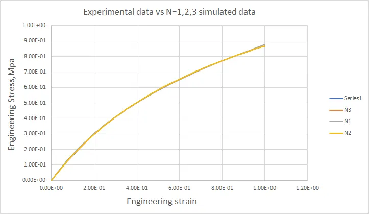
• From, the figure it is evident that the simulated data that are taken from the d3hsp files with the order of the polynomial N=2 & N=3 matches exactly with the experimental stress-strain data when compared to the order of polynomial N=1.As the order of polynomial increases, the fitted curves exactly match with the experimental stress-strain curves.

COMPARISON OF SIMULATED STRESS-STRAIN WITH EXPERIMENTAL STRESS-STRAIN DATA

For case 1: with the order of the polynomial N=0,

• Stress and Strain curve is plotted for the element which is there in the mid-portion of the specimen

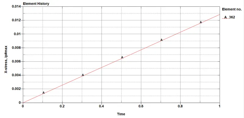
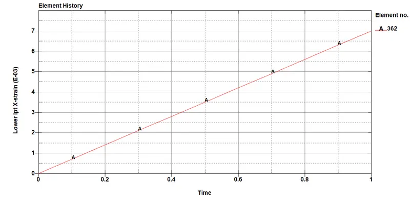
• Since these are True stress Strain values we can to convert it to Engineering Stress and Strain so that we can compare with the Material experimental data

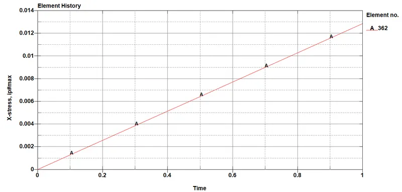
For case 1: with the order of the polynomial N=3,

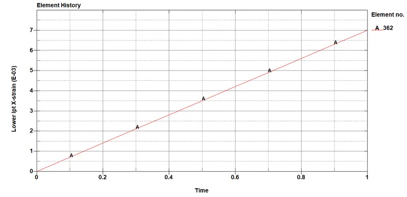
• Since these are True stress Strain values we can to convert it to Engineering Stress and Strain so that we can compare with the Material experimental data

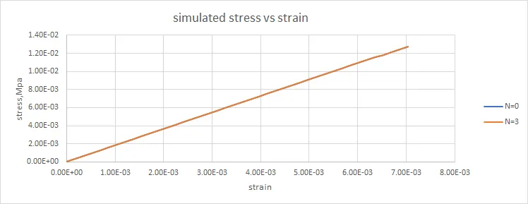
• when we compare, the simulated stress-strain data with the order of polynomial (N=0 & N=3), it is clear that our simulated curve behaves in a linear fashion since we have the stretch which is linear and whereas if we look at the experimental stress-strain data we see that their curves are somewhat curvy and this is due to actual testing of the material with the actual material properties and so the experimental stress-strain data differs from the simulated stress-strain data.

OGDEN MATERIAL

• The OGDEN Material constants for each case are stored in the d3hsp file

For first-order polynomial, N=1

mu(1)= 9.1076024661337E-01

alpha(1)= 1.3427238801352E+00

Final Fit Data from the d3hsp file is generally in Stretch vs True Stress but We have to Covert them into Engineering Strain vs Engineering Stress

Engineering Strain = Stretch -1

Engineering Stress = True Stress/(1+Engineering strain)

For first-order polynomial, N=3

Hyperelastic Constant C10= 0.2595E+00

Hyperelastic Constant C01= 0.4594E-01

Hyperelastic Constant C11= -0.2092E-01

Hyperelastic Constant C20= 0.2914E-02

Hyperelastic Constant C02= 0.1016E-02

Hyperelastic Constant C30= 0.0000E+00

For first-order polynomial, N=5

Hyperelastic Constant C10= 0.2611E+00

Hyperelastic Constant C01= 0.4420E-01

Hyperelastic Constant C11= -0.6074E-02

Hyperelastic Constant C20= -0.2667E-02

Hyperelastic Constant C02= -0.9968E-02

Hyperelastic Constant C02= -0.9968E-02

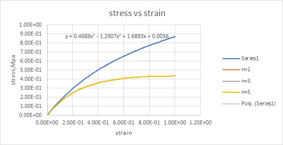
By Comparing, the 1st, 3rd, and 5th Order of polynomial Final Fit data they are very similar but they are very deviated from the Experimental data. so we will compare the Simulated Stress/Strain curve from the Tensile Test for Each order of the polynomial and check which Order of polynomial is better.

COMPARISON OF SIMULATED STRESS-STRAIN WITH EXPERIMENTAL STRESS-STRAIN DATA

For case 1: with the order of the polynomial N=0,

• Stress and Strain curve is plotted for the element which is there in the mid-portion of the specimen

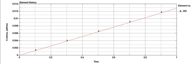
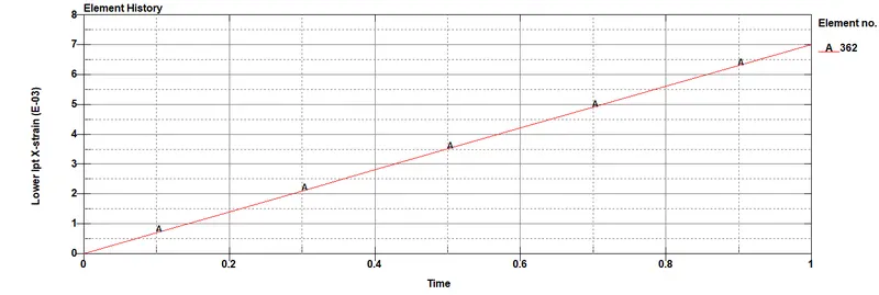
• Since these are True stress Strain values we can convert them to Engineering Stress and Strain so that we can compare them with the Material experimental data

For case 2: with the order of the polynomial N=5,

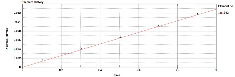
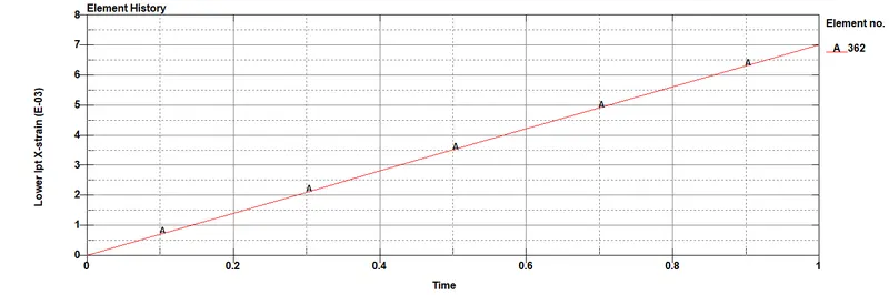
• Since these are True stress Strain values we can convert them to Engineering Stress and Strain so that we can compare them with the Material experimental data

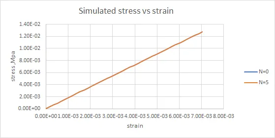
• when we compare, the simulated stress-strain data with the order of polynomial (N=0 & N=5), it is clear that our simulated curve behaves in a linear fashion since we have the stretch which is linear and whereas if we look at the experimental stress-strain data we see that their curves are somewhat curvy and this is due to actual testing of the material with the actual material properties and so the experimental stress-strain data differs from the simulated stress-strain data.

CONCLUSION

• we have created and modeled hyperelastic models and evaluated material constants for two models.
• With the help of material constants, we fitted stress-strain curves for different orders of polynomial from the d3hsp file and compared those strain curves with the experimental stress-strain curve for both hyperelastic models.
• Finally, we simulated a tensile test for both the hyperelastic models and obtained stress-strain data for different order polynomials and we converted them into engineering stress-strain data and plotted them. Finally, we compared the stress-strain curve of a simulated test model with the experimental stress-strain curve.