Week - 10 Hyperelastic Material Models
Aim:
- To perform the simulation and validate the curve as shown in the figure
Objective:
- To calculate and compare the Mooney Rivlin, Ogden material constants using stress-strain data by 100 percent strain
- From the above condition simulate and validate the material model using MPa(mm/ms)
- Finally, compare the d3hsp file from the simulation
Hyper-elastic Material:
- Hyperelastic material models are regularly used to represent the large deformation behavior of materials with FEA. They are commonly used to model mechanical behaviors of unfilled/filled elastomers.
- In addition to elastomers, hyperelastic material models are also used to approximate the material behavior of biological tissues, polymeric foams, etc. Linearly elastic materials are described through two material constants (Young’s modulus and Poisson ratio).
- In contrast, hyperelastic materials are described through a strain-energy density function. The strain-energy density can be used to derive a nonlinear constitutive model (i.e., stresses as a function of large strain deformation measures like deformation)
- Those are derived by researches and some acceptable models we are using popularly such as
Ogden
Neo-Hookean
Arruda-Boyce
Yeoh and Fleming
Mooney-Rivlin and Signorini models
Mooney Rivlin
The strain energy density function for an incompressible Mooney–Rivlin material is defined below. Where `C_ij>C_ij` are empirically determined material constants, I1 and I2 are the first and the second invariant. By varying the Index values of i and j we can change the constitutive equations and use them appropriately for our component. Similarly, we will be having multiple coefficients C
This changing of the index will be basically changing the order of the polynomial of the energy density equation. We need to find out the coefficients of these material models for a different order of the polynomial and extract the best fit curve data from the D3HSp file and compare it with the material curve
Ogden Material
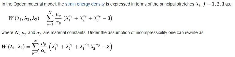
The Ogden material model is a hyperelastic material model used to describe the non-linear stress–strain behavior of complex materials such as rubbers, polymers, and biological tissue. The model was developed by Raymond Ogden in 1972. The Ogden model, like other hyperelastic material models, assumes that the material behavior can be described by means of a strain energy density function, from which the stress–strain relationships can be derived
Procedure:
Drafting Data
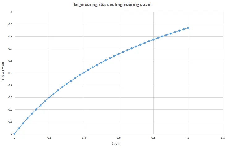
- The given Engg stress and Engg strain data of hyperelastic material is plotted in an excel sheet

Load curve
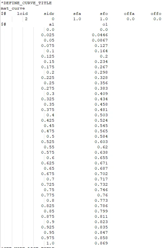
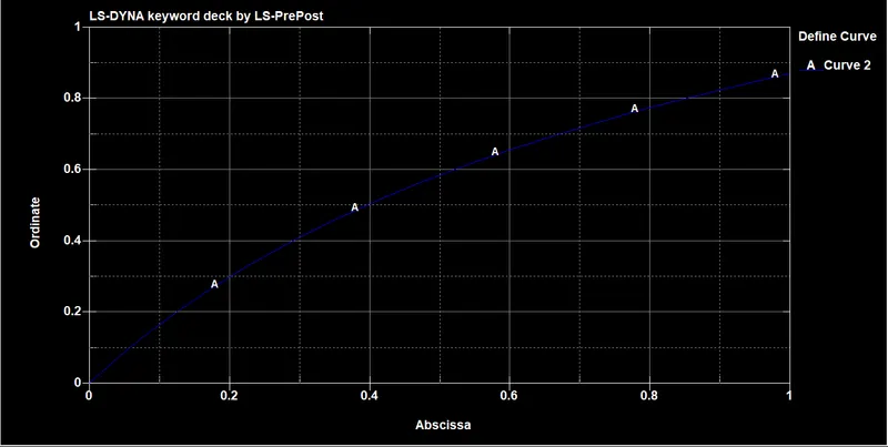
- The term material curve is assigned by defining a curve using a given engineering strain and stress plot
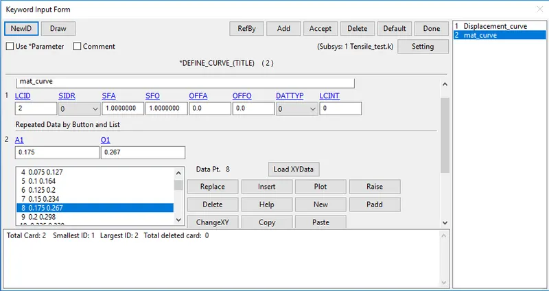
Material
- To check and validate the given material data with material models of Mooney-Rivlin, Ogden a dogbone specimen is taken for the analysis
- To find the Mooney-Rivlin and Ogden constants the value of N is set to 1-3. The value of density and Poisson’s ratio is taken as the generic value for the rubber material
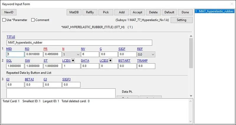
- The parameter N in the Mat_077(H) cards refers to the order of polynomial for which the constants are required to solve
This involves N1, N2, and N3 cases where the constants are solved along with stretch and true stress data - N1 solves for two polynomials C10, C01
- N2 solves for six polynomials C10, C01, C11, C20, C02, C30
- N3 solves for six polynomials C10, C01, C11, C20, C02, C30
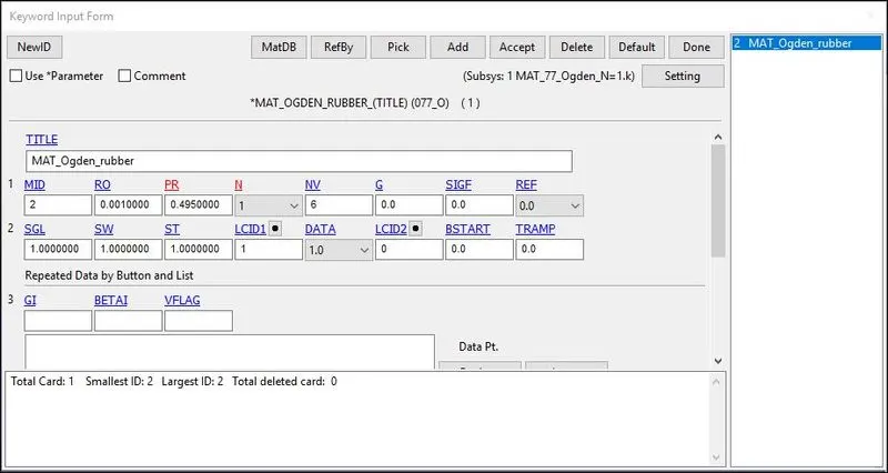
- The parameter N in the Mat_77(O) cards refers to the order of polynomial for which the constants are required to solve
This involves N1, N2, up to N8 cases where the constants are solved along with stretch and true stress data
The SW, SGL, and ST parameters are set to unity since we have a stress-strain load curve whereas in the case of force-displacement data requires specimen dimensions
Section
-
The section property of the dogbone specimen is assigned as a shell element with 1 mm thickness, ELFORM=2
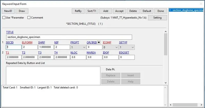
Part
-
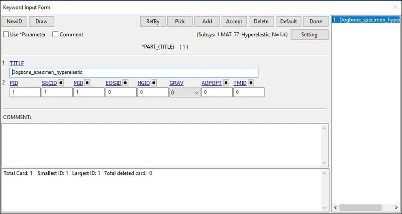
The Material and Section are assigned to the dogbone specimen part
Boundary Condition
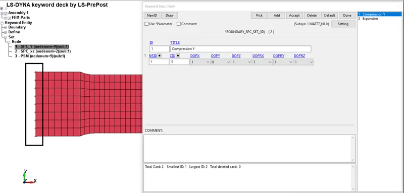
SPC
- The nodes at the fixed end are constrained in the X and Z direction only and the Y direction is not constrained because of lateral expansion during the tensile test
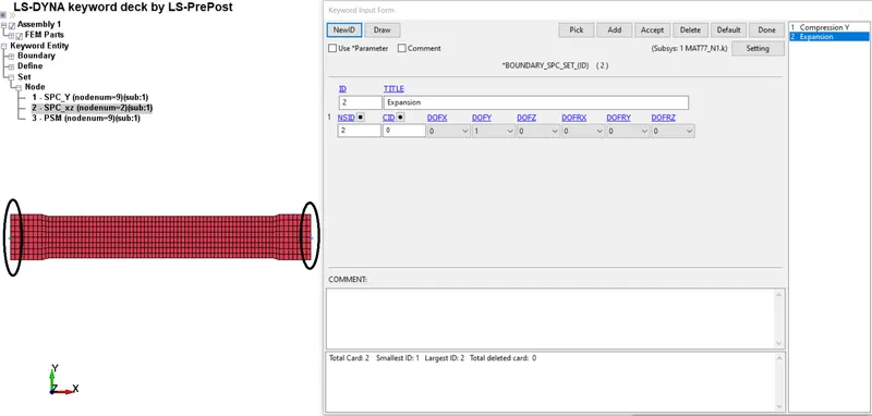
- The nodes at the middle are constrained in the Y direction since the neutral axis passes through the middle of the specimen in the X-direction
Prescribed motion
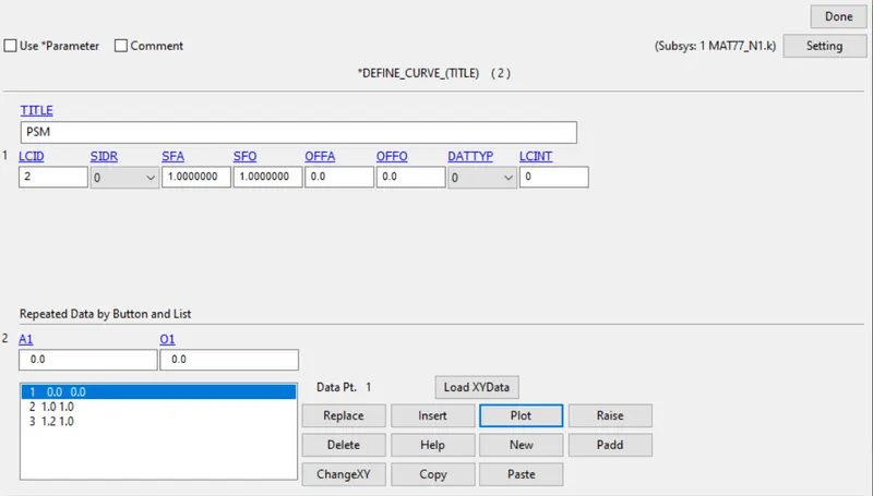
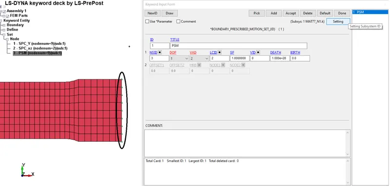
- PSM is created at the opposite end by specifying the displacement nodes using the Load curve LCID. Since the given stretch ratio is 100%
`epsilon = lamda - 1`
`lamda = 2, rarr epsilon = 2 - 1 rArr 1`
`epsilon rarr (dell)/L = 1, L=145`
L = 145
Control Cards
- To activate implicit analysis and define associated control parameters. The following keyword is required for all implicit analyses
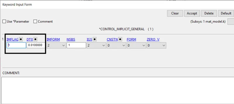
- IMFLAG: Implicit/Explicit analysis type flag: 1- Implicit analysis
- DT0: Initial time step size for implicit analysis: 0.010000
- IMFORM: Element formulation flag for seamless spring back: 2 retain original element formulation (default)
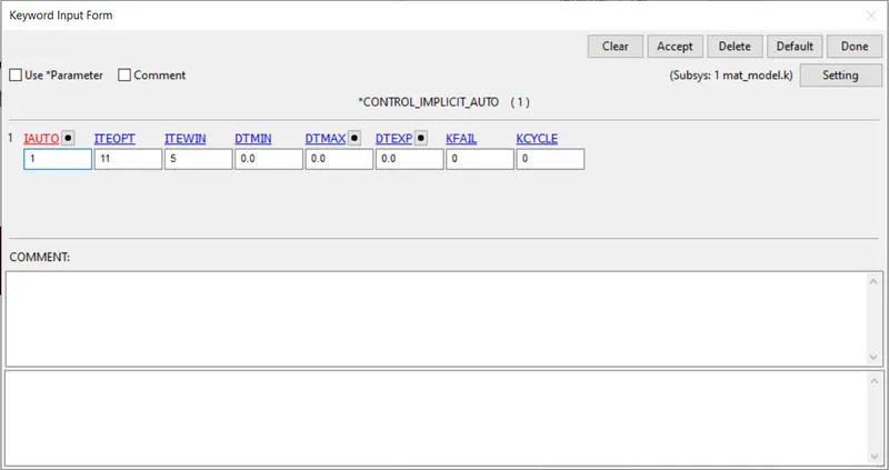
IAUTO: set to 1 which automatically adjusts the timestep size
ITEOPT: optimizes the operation count step 11
ITEWIN: is the iteration window 5
DTMIN: Minimum allowable time step size 0
DTMAX: Maximum allowable time step size 0
Database 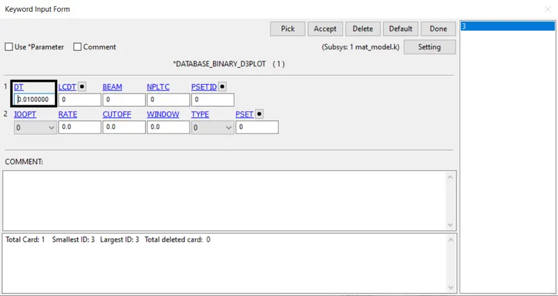
- BINARY_D3PLOT: It defines the frequency at which the animation file is to be created and is set to 0.01 ms
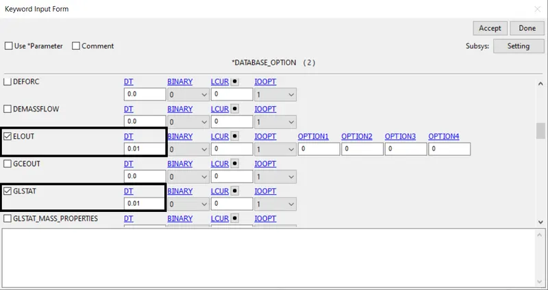
- DATABASE_ASCII_Option: The output request in ASCII format, The following keyword is activated
- ELOUT: Element Output Data and
- GLSTAT: Global Data
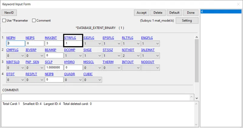
- DATABASE_EXTEND_BINARY: It plots the strain tensor to d3plot when STRFLG is set to 1
Results
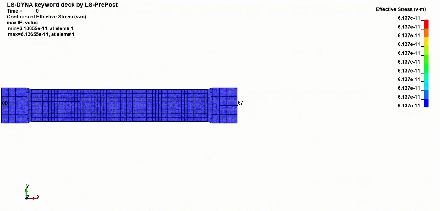
CONTOURS PLOTS OF X-STRESS
Material cases
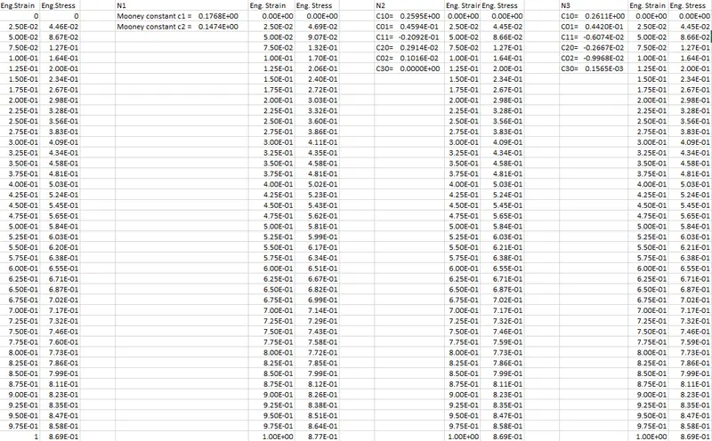
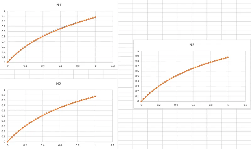
- From the data obtained of the d3hsp file for different polynomial values i.e, (N=1,2,3)
- The curves are converted from True to Engineering data and plotted in excel with comparison to Given data
- It is observed from the graph, that the curves of the different polynomial are superimposing with the experimental data
Material Validation
- To validate we need to key in the constants (C10, C01, C11, C20, C02, C03) from the above simulation materials with N1, N2, and N3
- By switching N=0 usually by *MAT_HYPERELASTIC_RUBBER we can input any of the Mooney-Rivlin constants according to the above cases (we used N=3)
- From the obtained true stress and strain, the Engineering stress and strain values are calculated and compared with the original data from the material curve
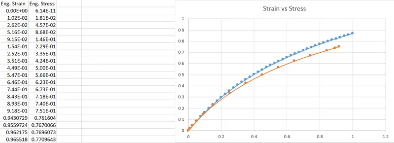
- From this data, we can easily found that the reduction in area is comparatively less for experimental hyperelastic than the original given data
- Due to some non-linearities, there could be some deviation that is agreeable compared to the original
Conclusion:
- The Mooney-Rivlin and Ogden material constants are obtained and verified from the d3hsp file
- By entering the value of polynomial N in the material card MAT_77_H the stretch vs stress curve data obtained and verified with experimental material data
- The simulation results of the tensile test for a material model show experimental data with slight deviation due to the high non-linear behavior with the help of generic values