Week 1- Mixing Tee
Aim :- Study of mixing effectiveness of fluids with different temperature flowing inside a pipe having T-junction using Ansys Fluent steady-state simulations.
Introduction -
Mixing Applications : The simulation of mixing 2 fluids having different thermal & physical properties have major application in vast areas,like chemical process industries & household air-conditioning etc.
Turbulence models : The Reynolds-averaged Navier–Stokes equations (or RANS equations) are time-averaged equations of motion for fluid flow, they are primarily used to describe turbulent flows.
Two equation model - it includes two extra transport equations to represent the turbulent properties of the flow. This allows a two equation model to account for history effects like convection and diffusion of turbulent energy. The first transported variable is turbulent kinetic energy -k. The second transported variable in this case is the specific dissipation `omega`or `epsi`. It is the variable that determines the scale of the turbulence, whereas the first variable, k, determines the energy in the turbulence.
K-epsilon model - is one of the most common turbulence models, although it just doesn't perform well in cases of large adverse pressure gradients.The K-epsilon model has been shown to be useful for free-shear layer flows with relatively small pressure gradients. Similarly, for wall-bounded and internal flows, the model gives good results only in cases where mean pressure gradients are small; accuracy has been shown experimentally to be reduced for flows containing large adverse pressure gradients. One might infer then, that the K-epsilon model would be an inappropriate choice for problems such as inlets and compressors.
K-omega SST model - is a two equation eddy viscosity model which has become very popular. The shear stress transport (SST) formulation combines the best of two worlds. The use of a k-ω formulation in the inner parts of the boundary layer makes the model directly usable all the way down to the wall through the viscous sub-layer, hence the SST k-ω model can be used as a Low Re-turbulence without any extra damping functions. The SST k-ω model does produce a bit too large turbulence levels in regions with large normal strain, like stagnation regions and regions with strong acceleration. This tendency is much less pronounced than with a normal k-ε model though.
Solution & comparision of different cases :-
Consider an air(fluid) flowing inside pipe, Cold horizontal-Y inlet is at 190C and hot vertical-X inlet is at 360C.Turbulent mixing of fluid of different temperature in T-junction & Outlet will be analysed at steady state.
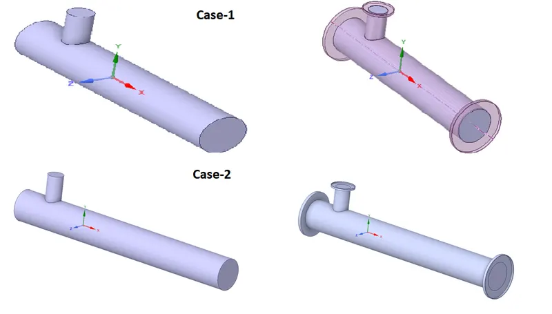
Case 1 : Short mixing tee
a) Momentum ratio - 2
Cold Inlet velocity - 6m/s
b) Momentum ratio - 4
Cold Inlet velocity - 12m/s
Case 2 : Long mixing tee
a) Momentum ratio - 2
Cold Inlet velocity - 6m/s
b) Momentum ratio - 4
Cold Inlet velocity - 12m/s
WorkFlow :-
(1) Geometry - Space claim
- Solid model in '.STEP or .SLDPT' format are loaded in Ansys space claim
- Fluid volume is captured using 'volume extraction' & by selecting edges of wet volume.
- Solid is then suppressed & hidden for further physical analysis.
T-junction pipe system in a vertical plane
(2)Setup Mesh
- In Ansys Mesh configuration are generated by default and we can view in & change the element size accodingly.
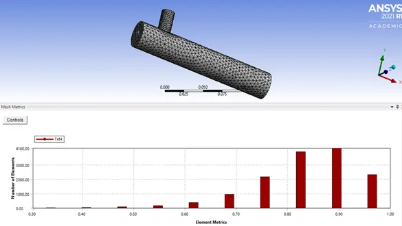
- 0.002m Fine grading Mesh grading is used to capture accurate results.
- Next, all the faces are named appropriately.

Mesh Quality :
Element size - 0.002, we can see that quality ranges from min 35% to max 95%.
12583 tetrahedral cells
2797 nodes
Observations
- When medium coarse mesh was used of 0.01element size mesh metrics in case-1 sort tee, all the solutions where going unstable or not converging.
(3)Setup Fluent:
- Setup is open in console window meshed file will be loaded & all configurations of model like mesh reading,building & distributing,setting volume, Zone etc. are done.
- We can perform mesh check & evaluate options to confirm orthogonality.
- In solver options, will select 'type - pressure based' , 'velocity formulation - Absolute' &'Time - steady'.
- Under physics, will select Energy as we are intersted in finding the thermal gradient results.
- Material is set to air only throughout fluid volume.
- Later boundaries are defined for Inlet velocities & temperatures.
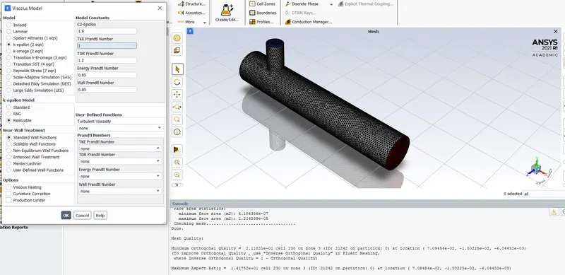
Case 1(a) : here will use two types of Viscous models approaches to solve Eqns. & compare for same case1(a).
After hybrid Intialization successful run & now we can start the iterations / solution convergence by input of appropriate no. of iterations and click on calculate to run iterations.
i) k-epsilon realizable std. model :-
Scaled Residuals -
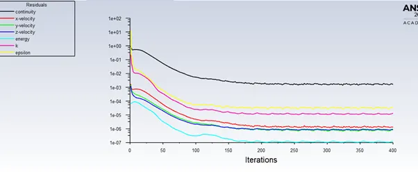
Solution found not converging(going infinite iterations) to steady state in the K-epsilon realizable model ,as we can see in that above plot that residuals are continously repeating.
Therefore, K-Omega SST model will be used for all cases.
ii) k-omega sst model :-
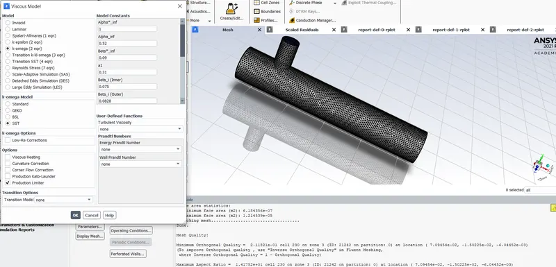
Elementary statistics feature in Ansys solution is used to generete reports of output variable & also to check the transient behaviour.
(4) Solution reports :
Scaled residuals & solution convergence -
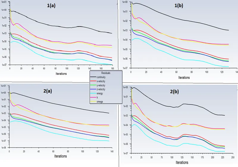
When Transport equations & physcial model equations are solved numerically , residuals propagation ideally should be zero & reducing during iterations. Form above convergence plot , we can see that velocity components are reducing gradually & Energy has least values,espically in Long pipe- cases.
Average velocity at outlet -
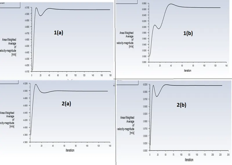
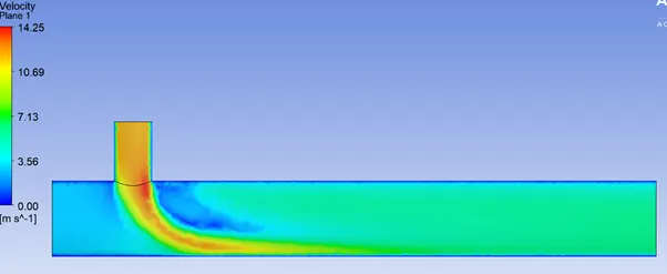
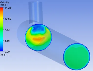
In case 1(b) we can pbsrve that there is no intial spike/higher value compared to other cases. It shows that short pipe with higher cold air Inlet there is uniform momentum available at outlet, indicating significant mixing before reaching outlet due to eddies & turbulence effects.But in all other cases, higher momentum is reached at very first few iterations.
Average temperature at outlet -
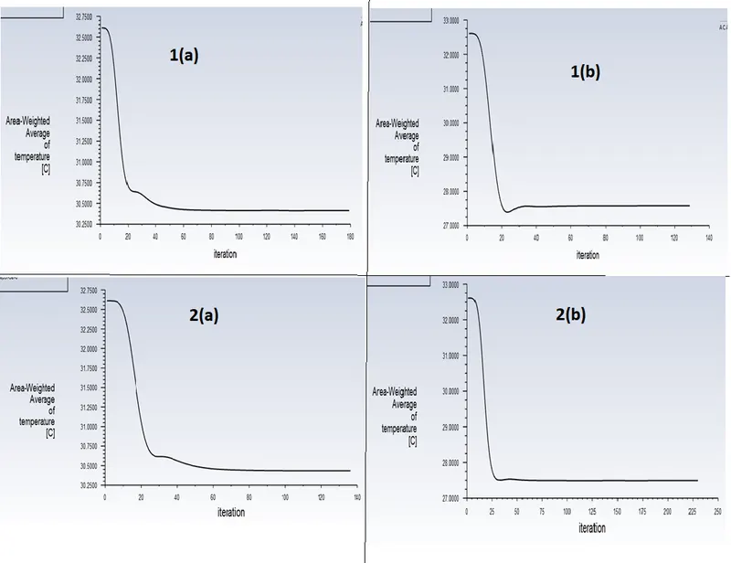
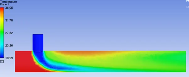
Lower temperature is achived in higher cold air Inlet velocity cases, but as Long pipe(2b) is showing similar result, 1(b) will be the efficient.
Standard deviation of temperature at outlet -
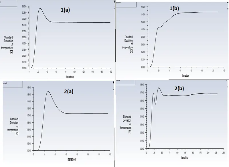
we can see that in case 2(b) there is a least deviation of temperature & thus effective mixing.
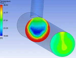
5) Results - post setup :
1(a)
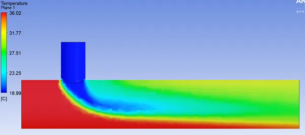
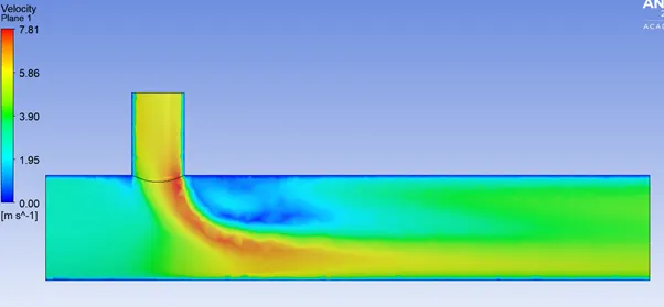
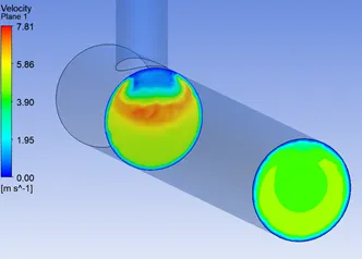
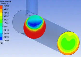
1(b)
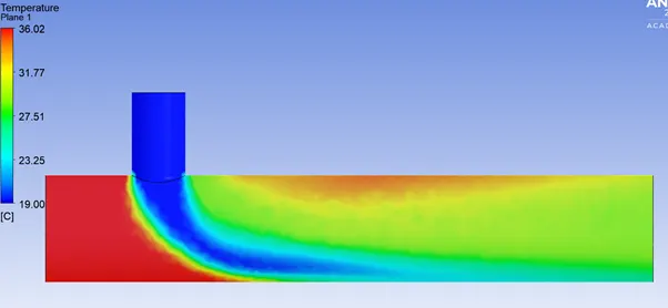
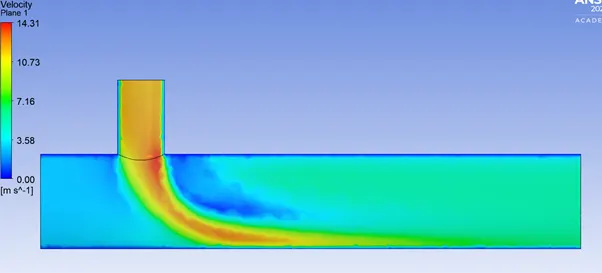
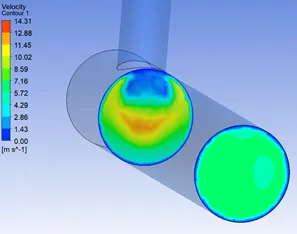
2(a)
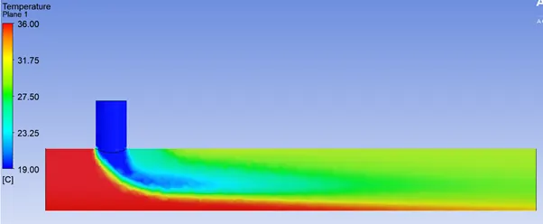
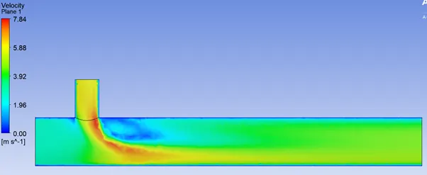
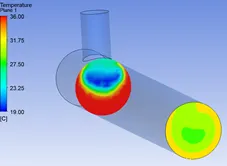
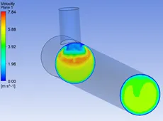
2(b)
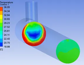
| simulation run time | No. of iterations | average temperature | |
| Case 1a | 201 sec | 179 | 30.4 C |
| Case 1b | 207 sec | 129 | 27.5 C |
| Case 2a | 153 sec | 136 | 30.45 C |
| Case 2b | 262 sec | 230 | 27.2 C |
Case1b took least no. of iteration compared others.
Theoretical calculation
Hot Mass flow `m^h`= `rho*A^h*V^h`
cold mass flow `m^c`= `rho*A^c*V^c`
Mometum ratio `Mr = V^c/V^h`
`A^h = 9.07 mm^2`
`A^c = 2.27 mm^2`
`T(mix) = (A^h*V^h*T^h + A^c*V^c*T^c)/(A^h*V^h + A^c*V^c)`
`= cancel(V^h/(V^h))((A^h*T^h + A^c*Mr*T^c)/(A^h + A^c*Mr))`
For case 1 - Mr = 2
`T(mix) =(9.07 xx 36 + 2.27xx19xx2)/(9.07 +2.27xx2) = 30.32 C`
For case 2 - Mr = 4
`T(mix) =(9.07 xx 36 + 2.27xx19xx4)/(9.07 +2.27xx4) = 27.49 C`