Week 1- Mixing Tee

AIMS : To understand the mixing effeciency of a tee joint under different conditions.

OBJECTIVES: 

• To find the suitabel model among k-epsilon and k-omega for this simulation.
• To  perfome a grid convergence study to use better mesh for the simulations
• Run the simulations for Case -1 and Case-2 and compare the results to understand the effect of momentum ratio length of the tee-joint . 
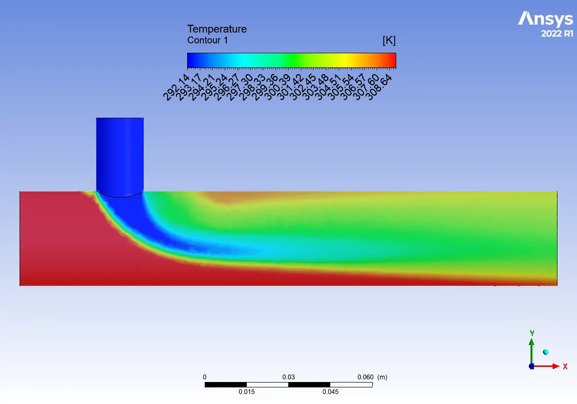
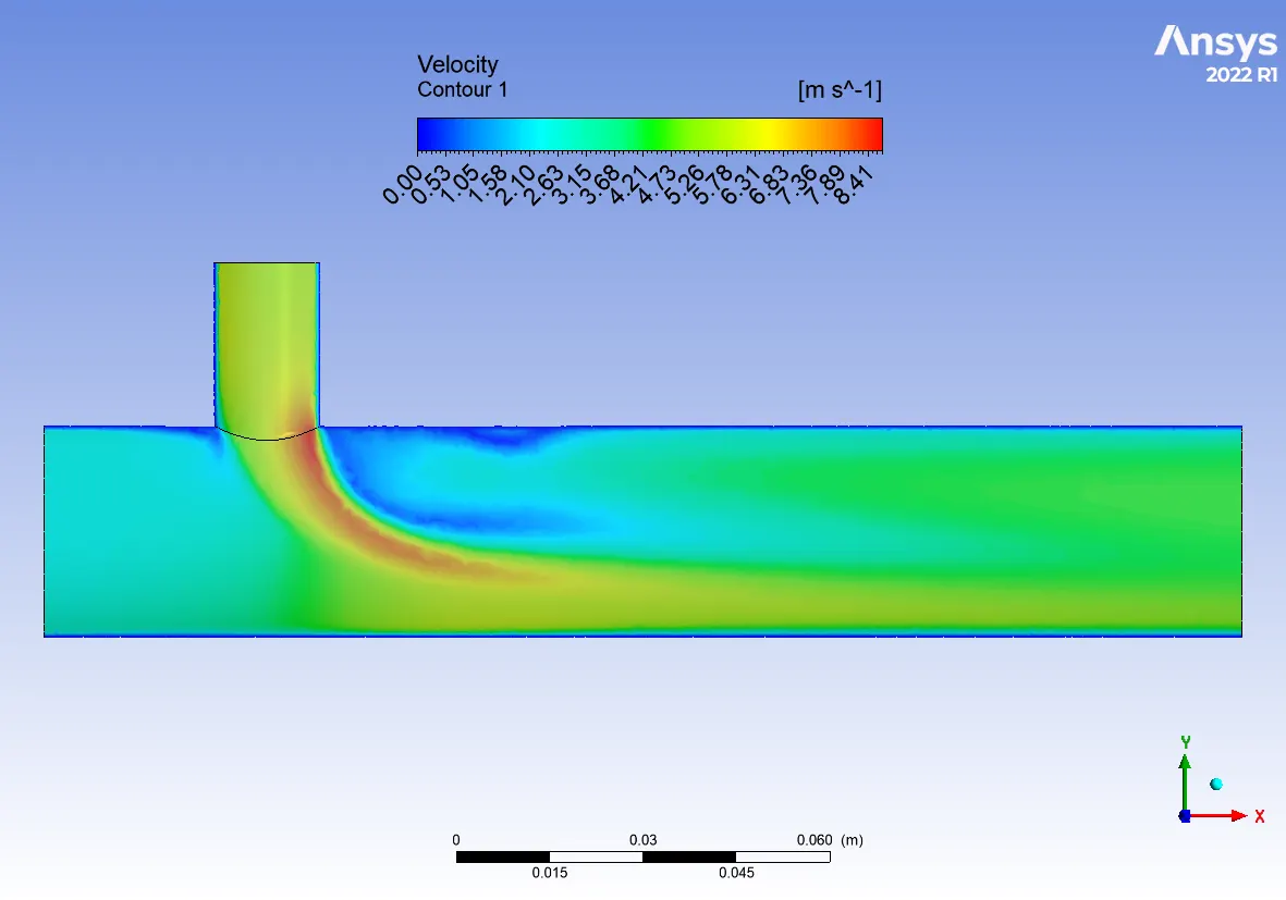
• Plot the temperature and velocity contours accordingly along with the average temperature and standard deviation values to understand the mixing effeciency of the cases. 

 

THEORY

Mixing Tee:

 Fluid mixing is represented in the form of mixing two coaxial jet flows with good mixing efficiency. It is generally used for applications that require an efficient mix of two fluid streams with different physical & chemical properties combination together to form one stream. For example, this mixing Tee is used in high pressurised application like an Air Conditioner. In the mixing of Fluids, thus viscosity is a prevailing property of the system mixing if it is in lower the value the turbulent mixing can be achieved quickly and mixing operation can be easily done. Moreover, the standard deviation method used to examine the mixing efficiency in tee simulation.

GEOMETRY 

Intially a two T-joint geometry was provided with different lengths. The geometry of the short T-joint is given below. Now the fluid volume was extracted as we do not need the extrented outer part. Using volume extract command in space cliam the required edges were selected and the volume was extracted. 

 

 

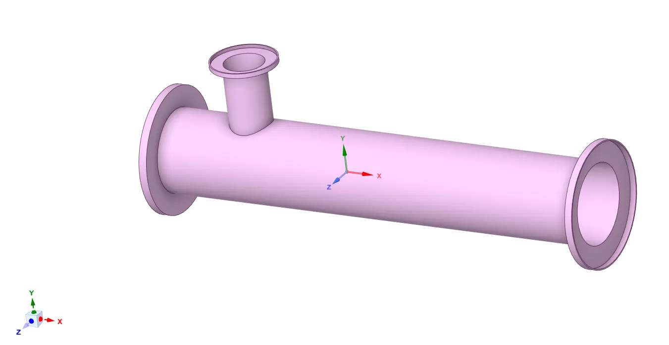
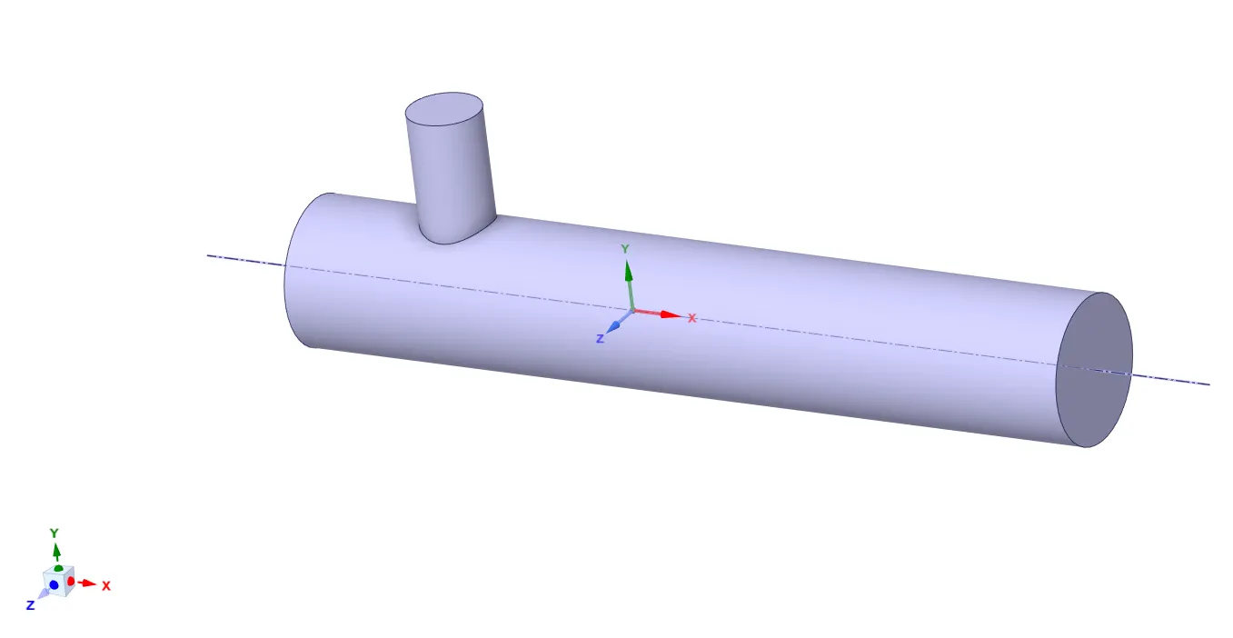
The figure below is the extracted volume which will be used to run the simulations for short T-joint. Similar process was used to extract the fluid volume from the long T-joint geometry. After extracting volume supress physics command was used to prevent the solid body involvement during meshing stage.

 

 

MESHING

 Now Meshing has been done using tetrahedral elements .In this whole simulation process 5 different meshes were generated . 

1. To find the suitable model between k-epsilon and k-omega a very coarse were taken with element size 0.025 to reduce the comuptational tome and effort . 

2. To perform the grid convergence test three different meshes were generated coarse , medium and fine with elements sizes  0.005 , 0.0025, 0.001 respectively. Through this the better perfoming mesh is used for Case-1 and Case-2 

3. Finally one more mesh is used for long -tee simulations with element size of 0.001 to compare the results with the short t-joint fine results. 

In all the meshes the mesh quality is above 0.2 which is enough to run simulations in fluent without any errors. 

 

 

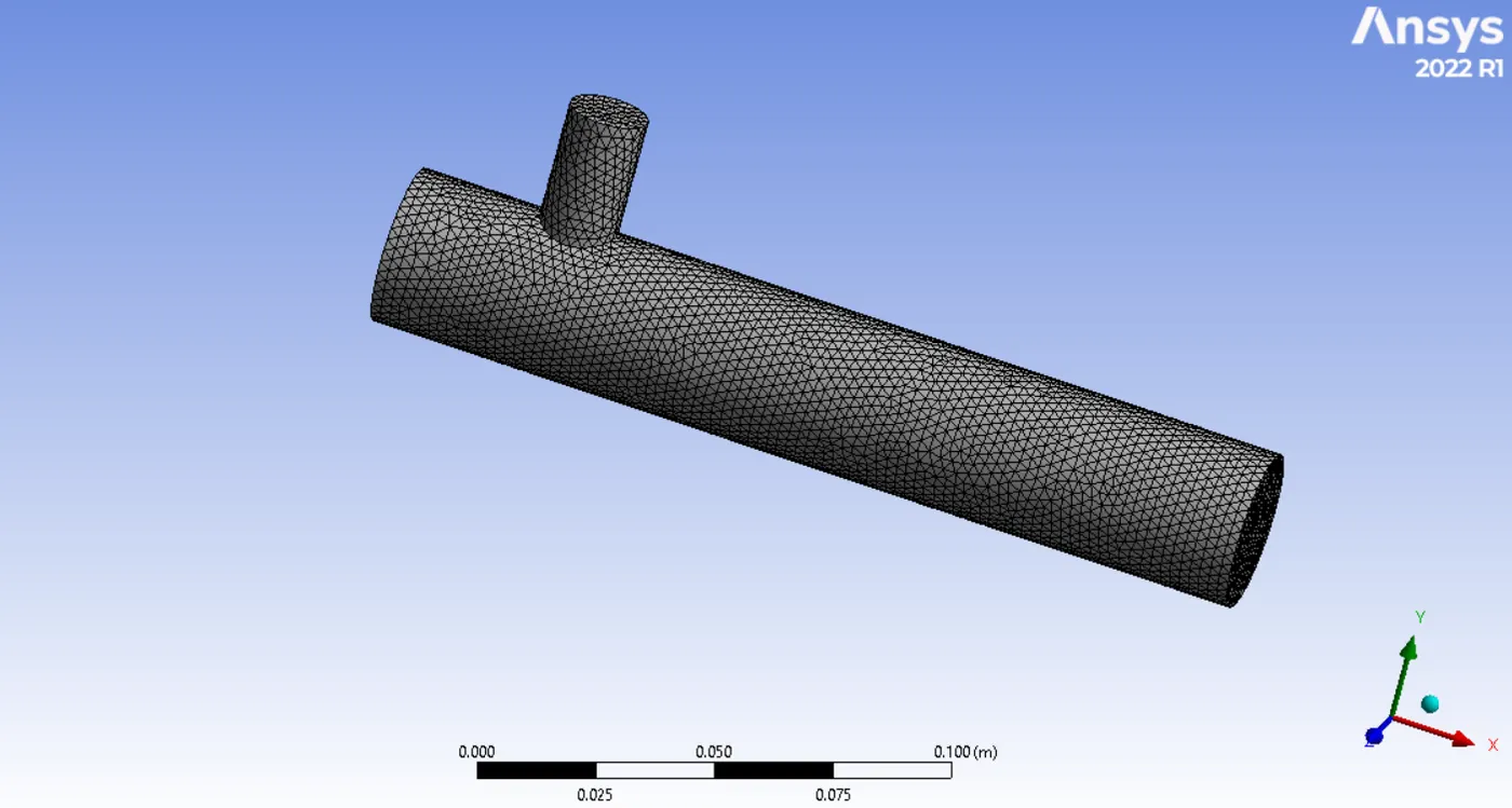
After the mesh is generated the boundary were named cold inlet, hot inlet. wall and outlet. Now the mesh is ready for simulation.

SET UP 

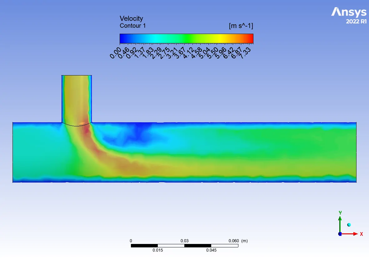
 To find better model for simulation

k-epsilon:

 

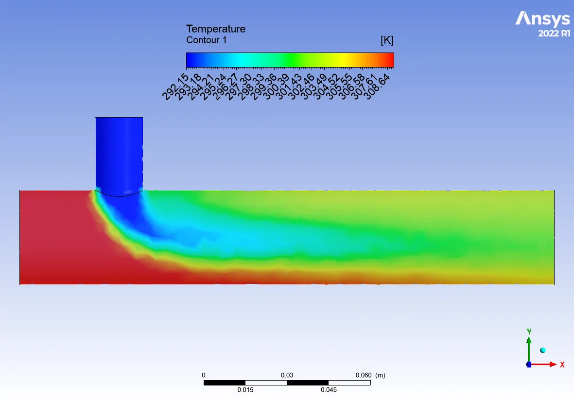
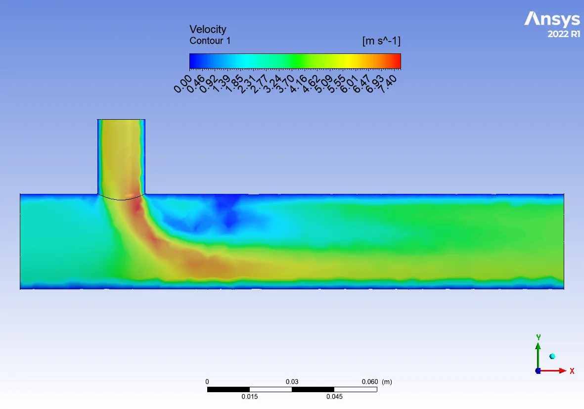
k-omega:

 

 

• In general, K-omega model is well suited for simulation flow in the viscous sub-layer. On the other hand, k-epsilon is ideal for predicting flow in the regions away from walls.
• The K-omega exhibit less sensitivity to the free stream conditions than any other turbulence models.  

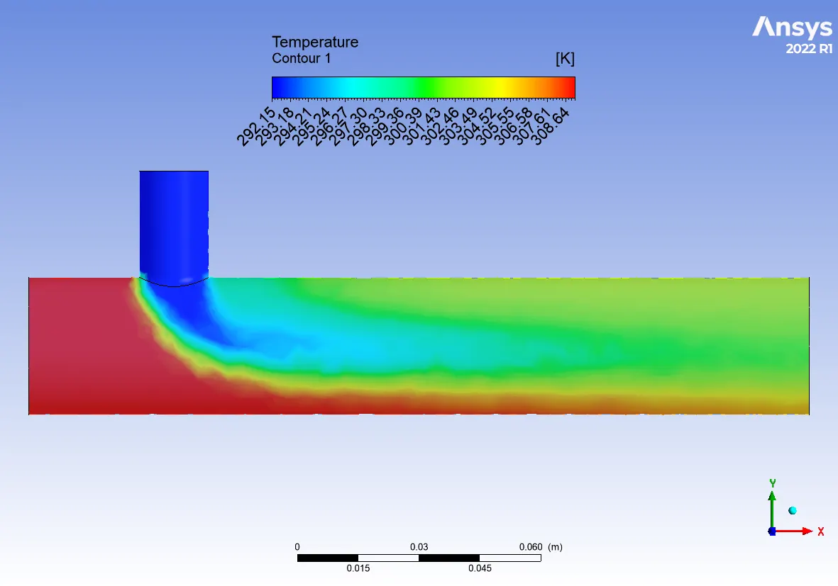
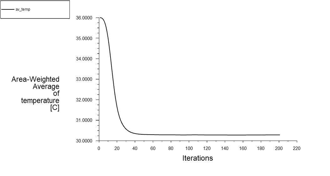
But in our case even though were not using the Y+= 1 to apply K-omega model  but for obtained average temperature at the outlet (30.2 Celsius) the mixing effecieny for K-omega is better than K-epsilon as the standard deviation values are 1.19 and 1.49 respectively. So we are using K-omega model for the rest of the simulations.

 

To find better mesh for the simulation

Coarse 

 

 

 

 

 

 

Medium 

 

 

 

 

Fine 

 

 

 

 

 

 

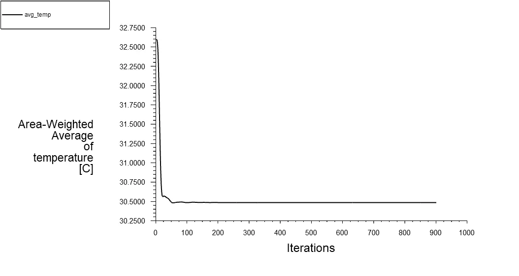
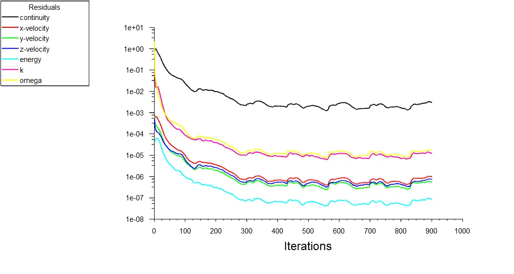
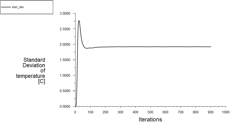
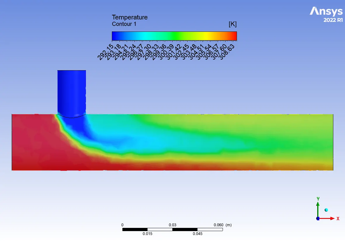
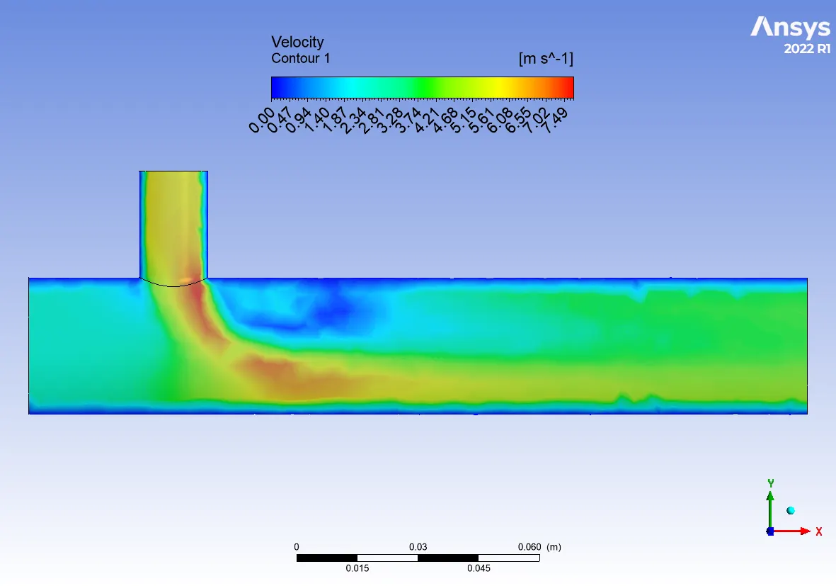
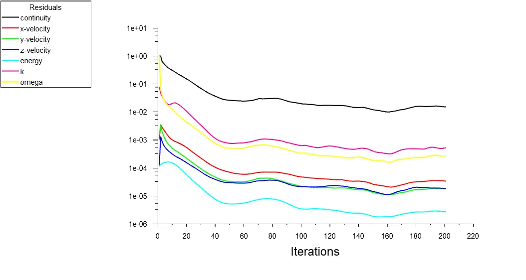
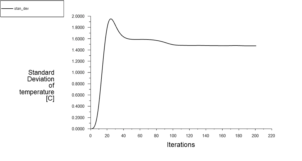
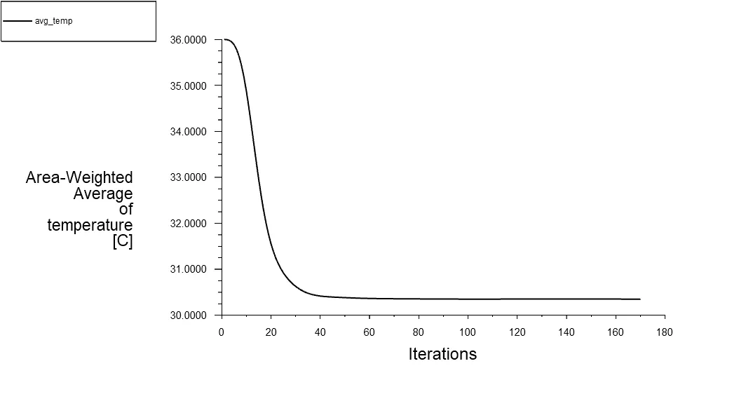
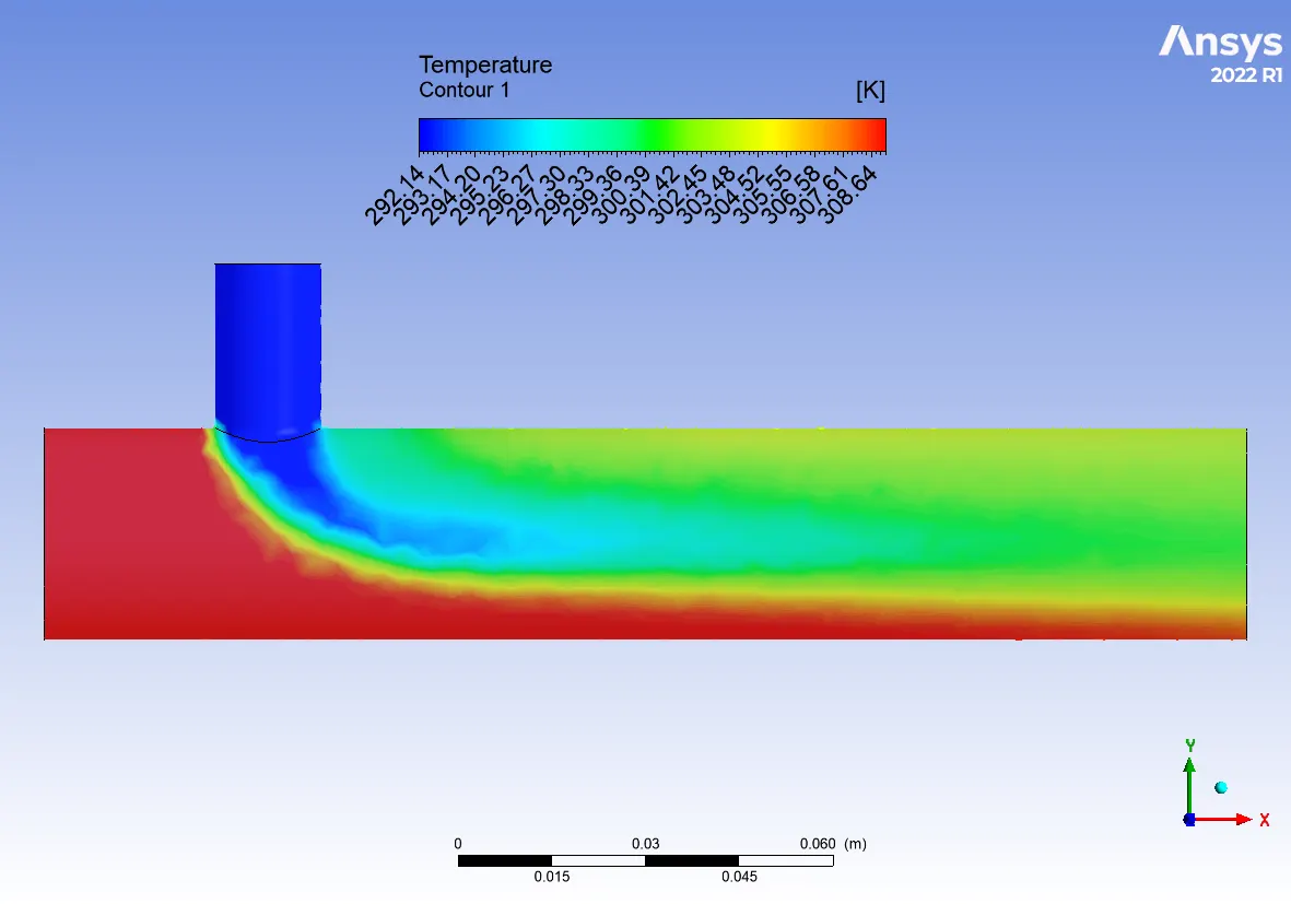
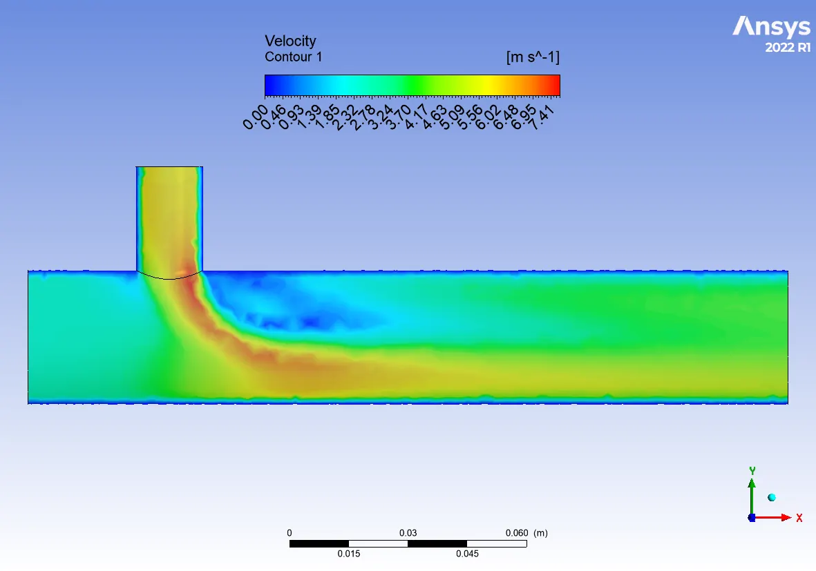
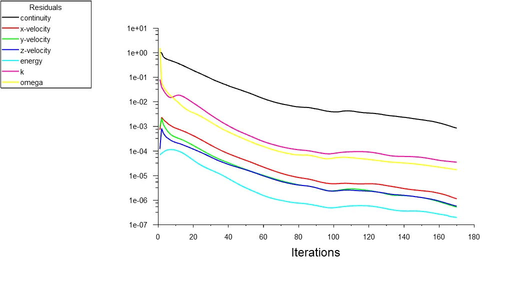
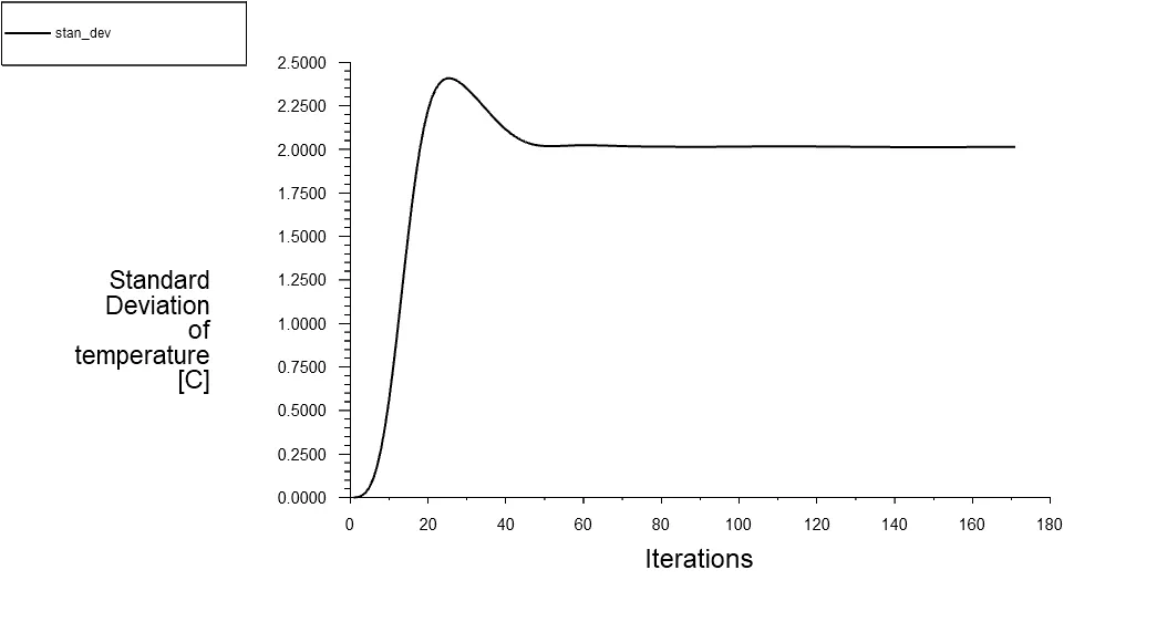
  The overview of the above prvided figures are presnted below in a table where we get a clear understanding on the coarse , medium and fine mesh results interms of average temperature at the outlet and the standard deivation, to understand the mixing efficiency. 

	Coarse	Medium	Fine
Element size	0.005	0.0025	0.001
Average Temperature	30.28	30.25	30.486
Standard deviation	1.47	2.01	1.91

From the above results we can see that almost all the meshes are providing similar results except fine a the mesh quaity is high the results obtained are being more precise . So fine mesh is choosen to continue with remaining simulations.

CASE-1 

ratio - 2 

 

 

 

ratio -4 

 

 

 

 

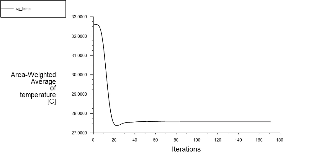
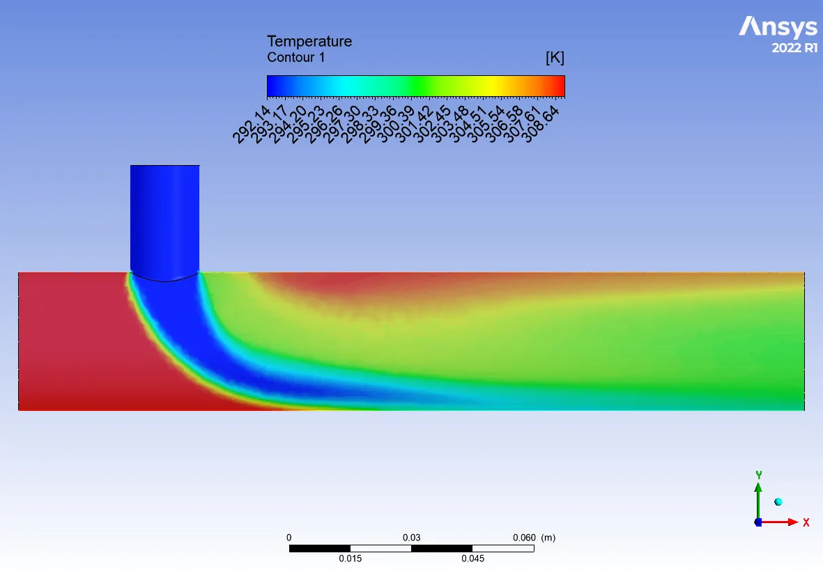
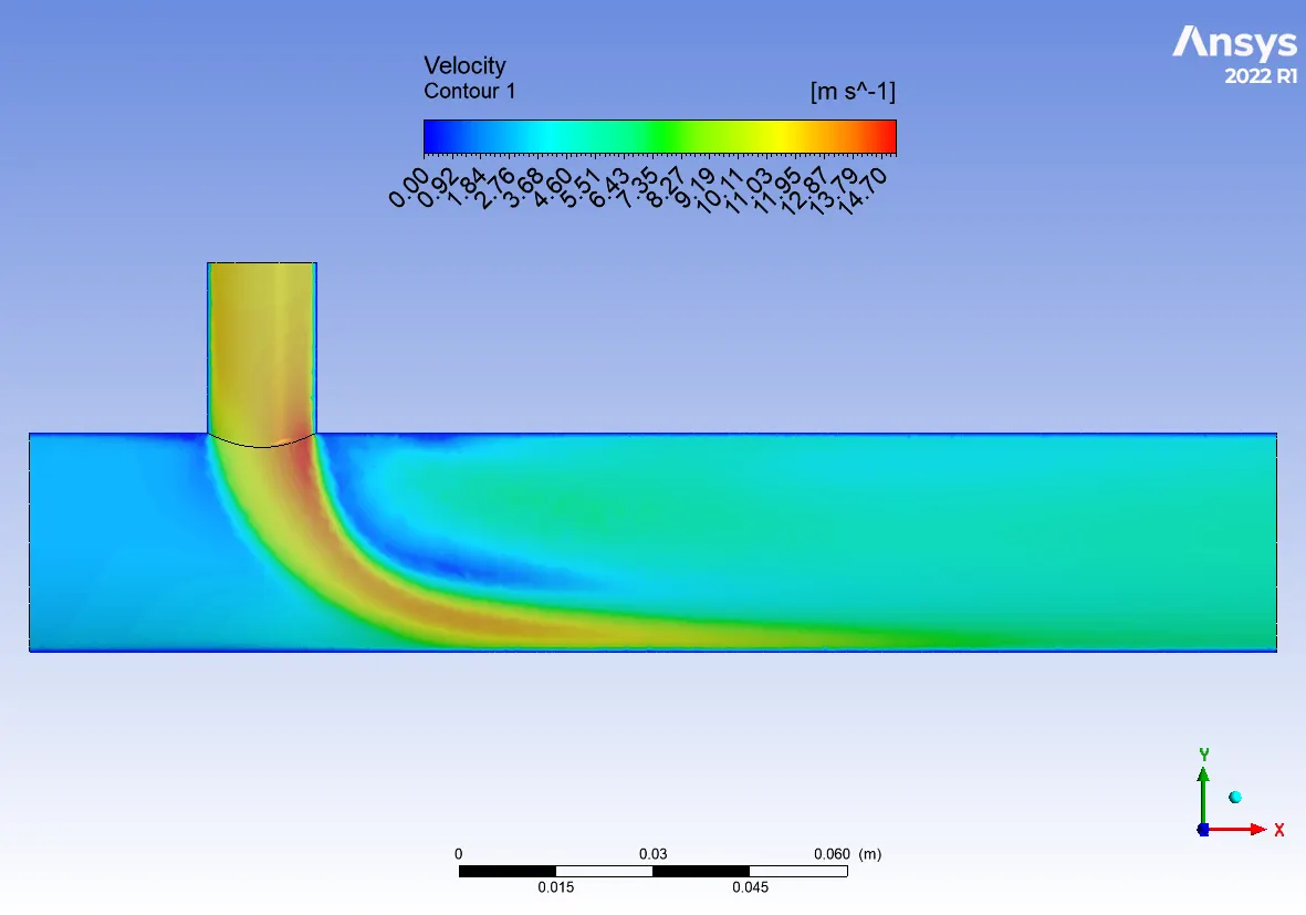
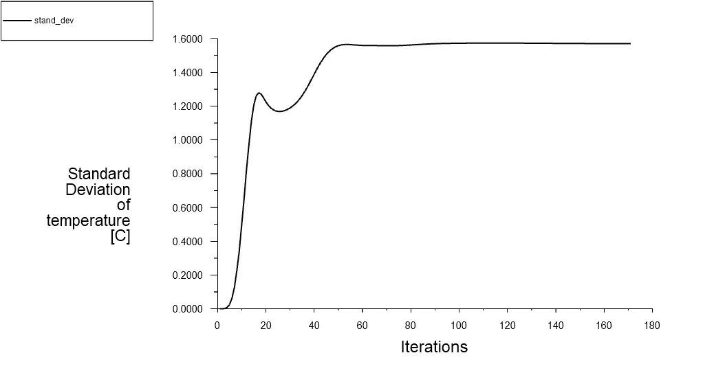
From the above figures we can understand that with increase in the speed of the cold inlet the mixing is being more effeicient. When the momentum ratio is 2 which means the hot inlet is 3 m/s and cold inlet is 6m/s the average temperature and standard deviation are 30.48 amd 1.91 respectively . When the ration is increased to 4 , which means the hot and cold inlet stream velocity are 3 and 12 respectively, the average temperature and standard deviation are 27.56 and 1.57 . 

 

 

Case-2

ratio-2 

 

 

 

ratio-4 

 

 

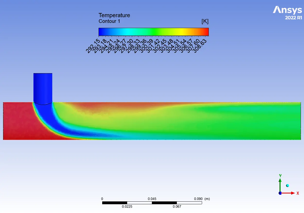
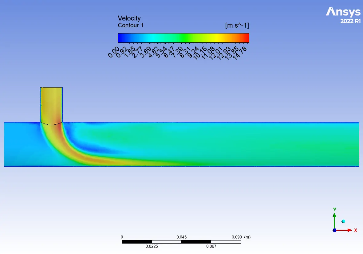
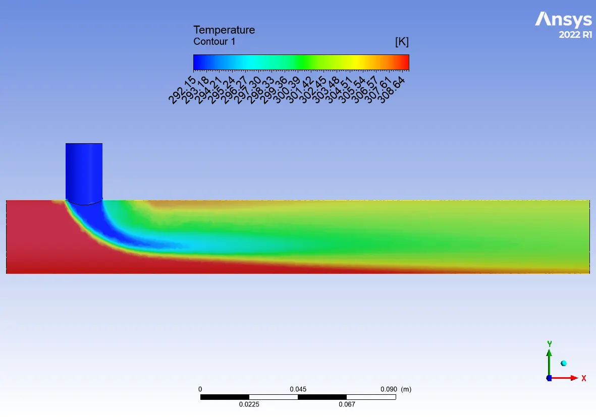
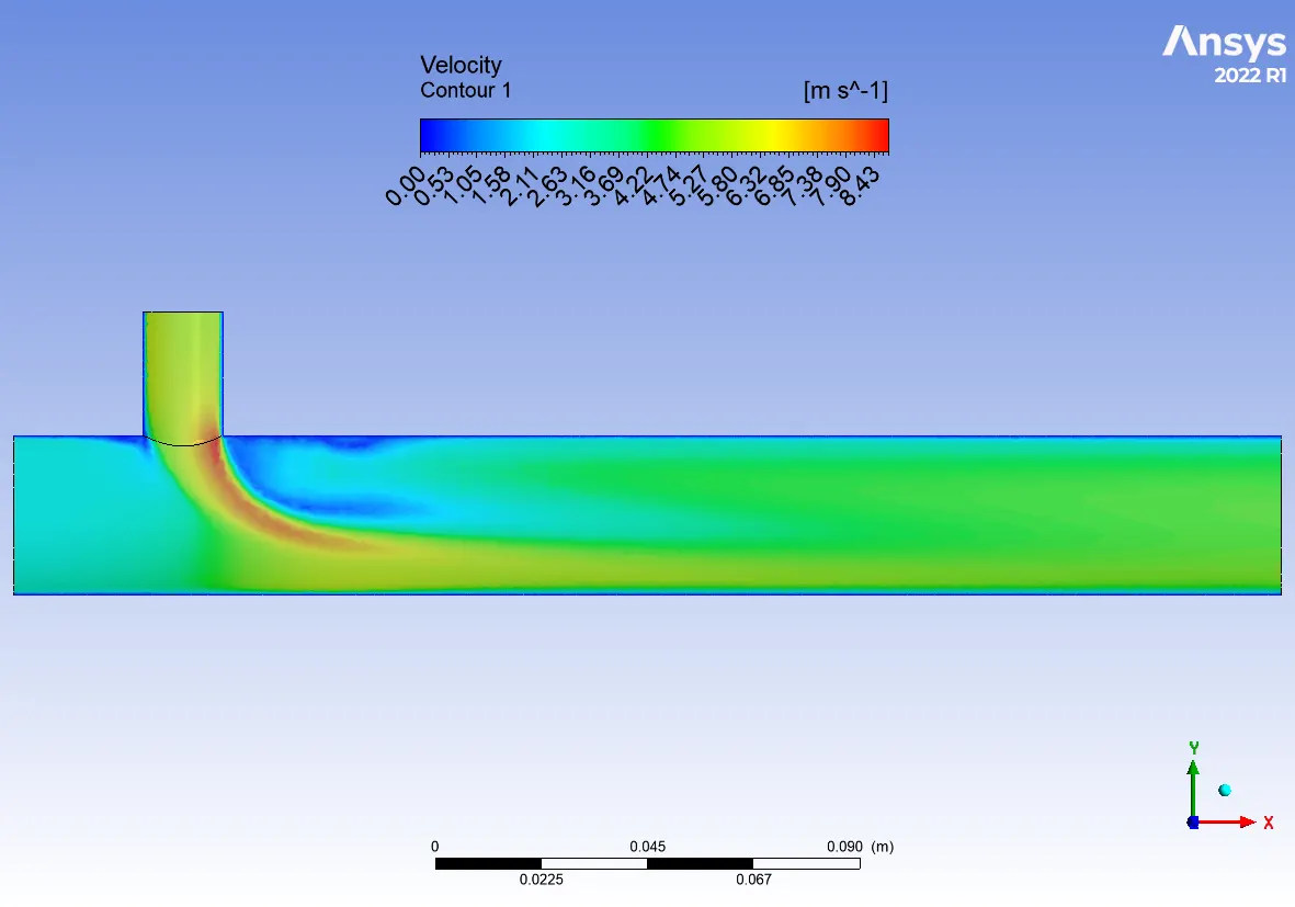
 In this case-2 we tried increasing the length the t-joint to see if there will be any significant changes in the mixing effeicienies and average temperature . But through the results obtained above we can obeserve the results are similar to the short tee joint results for both ratio 2 and ratio 4 . This can be clearly seen from the table provided below.

short -tee	cell count	average temp	convergence itr
ratio-2	576190	30.48	250
ratio-4	576190	27.56	267
long-tee
ratio-2	765896	30.47	336
ratio-4	765896	27.54	380

CONCLUSIONS:

1. From the results found k-omega is provided better mixing efficiency  than k-epsilon for obtained average temperature. 
2. After conducting simulations, as element number increases the convergence time also increases.
3. To get better mixing at outlet high velocity of flow is very effective. Therefore, a higher momentum ratio gives better mixing of hot and cold fluid streams at the outlet.
4. Finally, in the above case, it is very important to use a short mixing tee with a momentum ratio of 4 to get precise results.