Week 1- Mixing Tee
AIM:
To setup the steady state simulation to compare the mixing effectiveness of the fluid having various temperature and velocity in the tee joint. Have to find out the suitable model for performing the fluid flow. And to perform the flow for various cases provided and to compare these cases based on the cell count, average outlet temperature and number of iterations for converge. And also to provide the temperature contour, temperature line plot, velocity contour, velocity line plot for all these cases with their results.
THEORY:
Fluid mixing is represented in the form of mixing two coaxial jet flows with good mixing efficiency. It is generally used for applications that require an efficient mix of two fluid streams with different physical & chemical properties combined together to form one stream. That is mixing of the hetreogenous solution to provide a homogenous solution that is used for particular application.
The major application of these project is carried out in Hydro thermal power plant, HVAC, mixing of drugs in a blood stream etc..,
INTRODUCTION:
Cases to be performed with the hot inlet temperature of 36 C and cold inlet temperature of 19 C.
- Case 1
- Short mixing tee with a hot inlet velocity of 3m/s.
- Momentum ratio of 2, 4.
- Case 2
- Long mixing tee with a hot inlet velocity of 3m/s.
- Momentum ratio of 2, 4.
First of all we need to choose the model in which the simulation is going to be solved. For that we have to conduct the study 1.
PROCEDURE:
Functional flow in the software:
- Initially we have to open the Ansys workbench. And in that page we have the drag the Fluid Flow(Fluent) in to the project space.
- Then by right clicking the geometry option we have to open the geometry in the space claim.
- Then we have to extract the volume in the geometry where we have to simulate the fluid flow. After the volume is extracted then we have to go for the Mesh.
- In the Meshing window we have to name the each and every part in the geometry where the fluid is under calculation. Then we have to feed the data like temperature velocity for each face.
- Then we have to do the meshing.
- After the mesh is generated we have to go for the Setup, where we have to choose the solver, parameters and the required plot results for the particular problem.
- We have to initialize the setup and start running the calculation. After the calculation and plots are taken, we have to review it and verify whether the output results will satisfy with the required output or not with numerical calculation.
- If everything is okay then we have to select the Results, where it can display the graph, plots required for summarizing the results.
Study 1: (Case 1 ---> K-Epsilon model)
In this study we have to choose the model for the simulation. For that we have to take the K-epsilon model and K-Omega model. And with the short tee geometry we need to perform the simulation and have to compare the results. Based of the results we have to further proceed for the other cases.
Parameters taken in study 1:
Model : K-Epsilon Model, Realizable, Standard Wall functions
Solver : Pressure-Based
Velocity formulation : Absolute
Time : Steady
Meshing : Automatically generated.
Considered the Energy model.
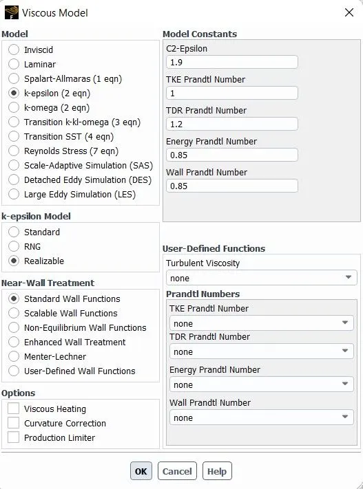
Input information for the study I:
Velocity at hot inlet - 3 m/s; Temperature at hot inlet - 36 C
Momentum ratio - 2
Velocity at cold inlet - 6 m/s; Temperature at cold inlet - 19 C
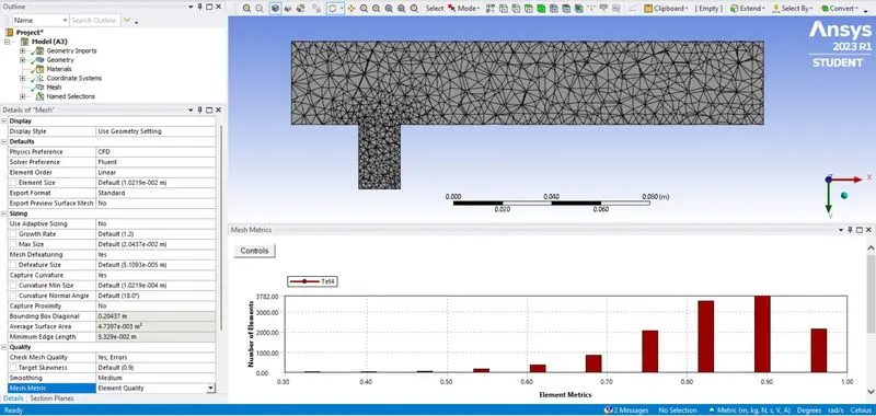
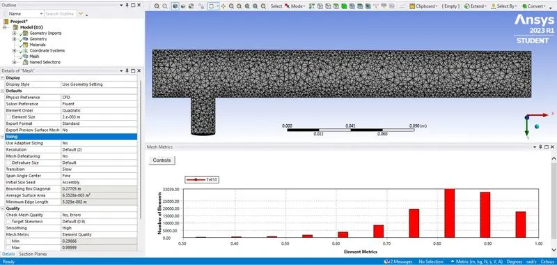
By providing the required inputs and choosing the exact parameters, meshing is done. And to show case the quality of the meshing element quality plot is also shown in the attached image.
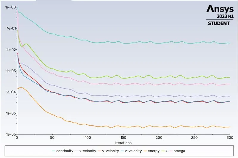
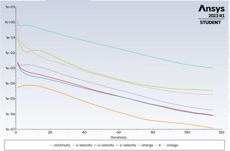
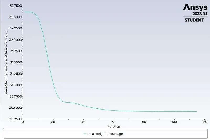
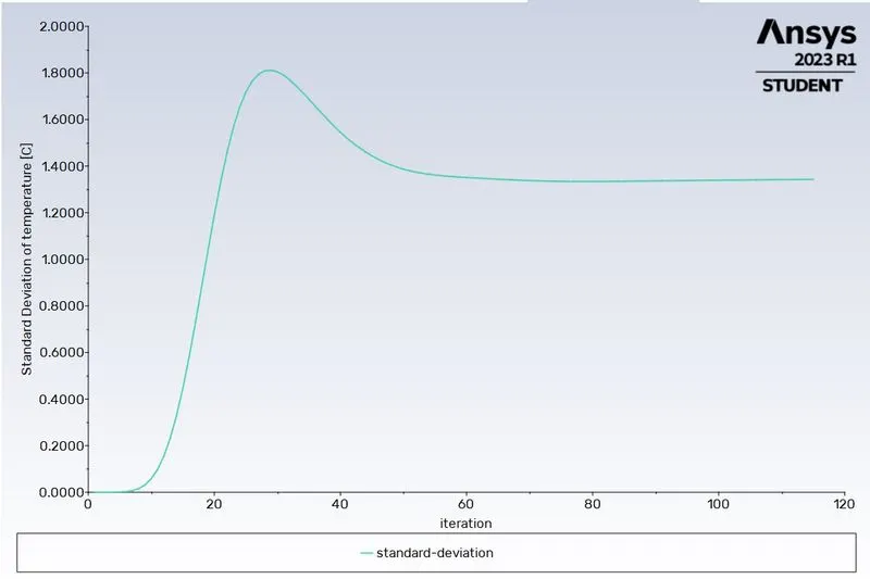
Then from the solution page we taken the scaled residuals plot, Area - weighted average plot, and the standard deviation plot.
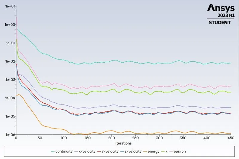
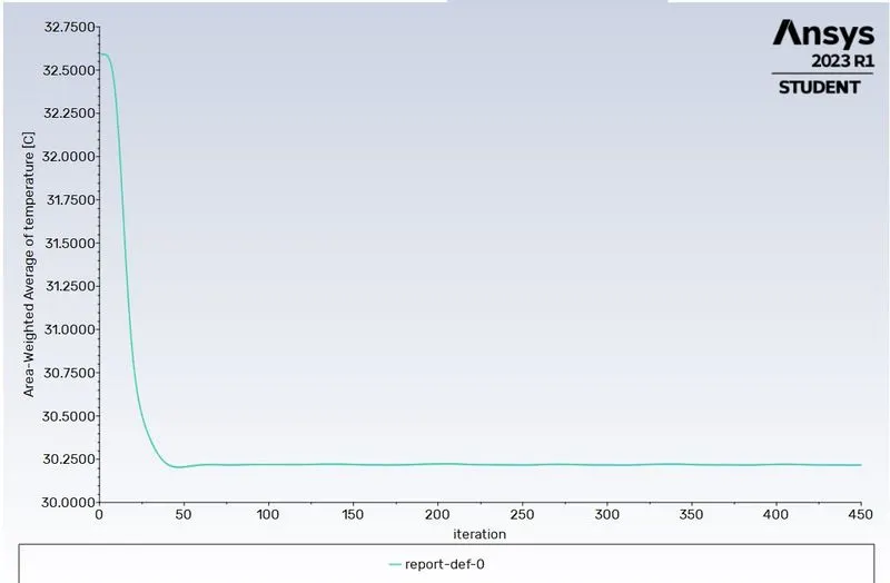
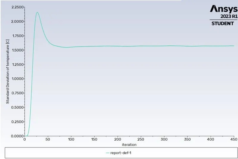
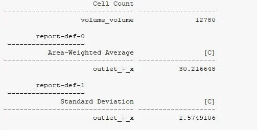
This is the result obtained for the mesh count, area weighted average for temperature at the outlet and standard deviation of the temperature.
Results Plot:
Temperature contour and respective plot along the pipe:
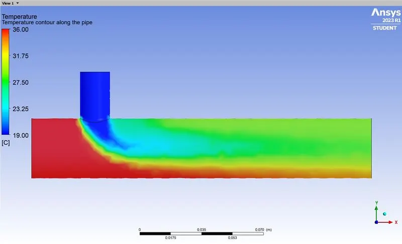
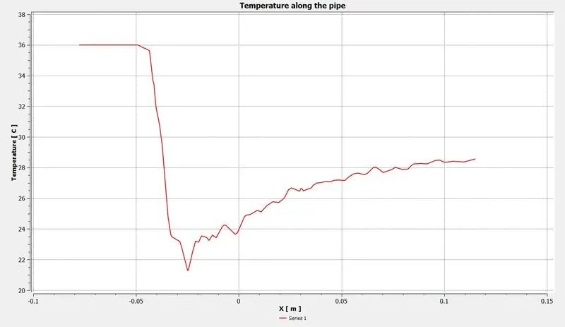
Temperature contour and respective plot across the pipe:
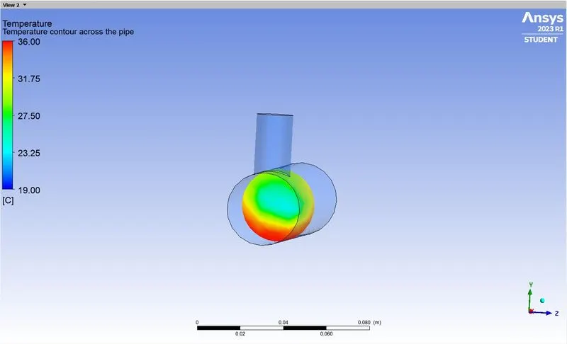
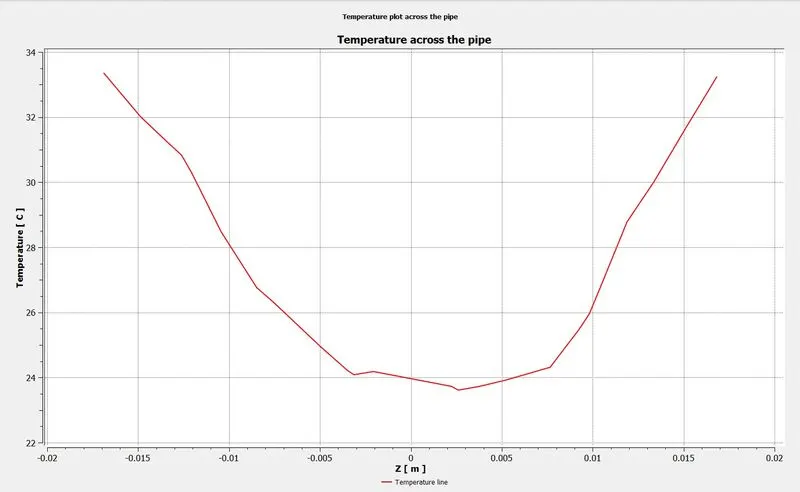
Velocity Contour and respective plot along the pipe:
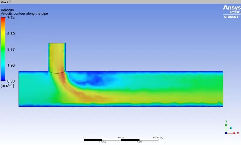
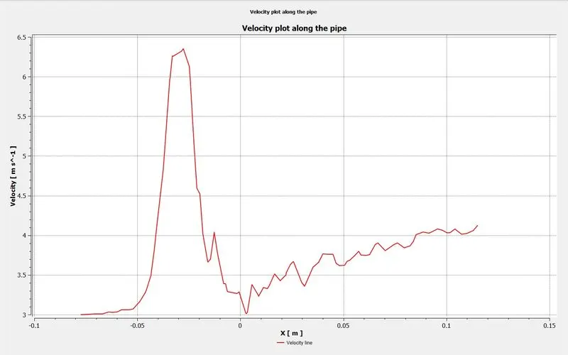
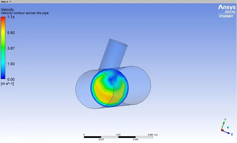
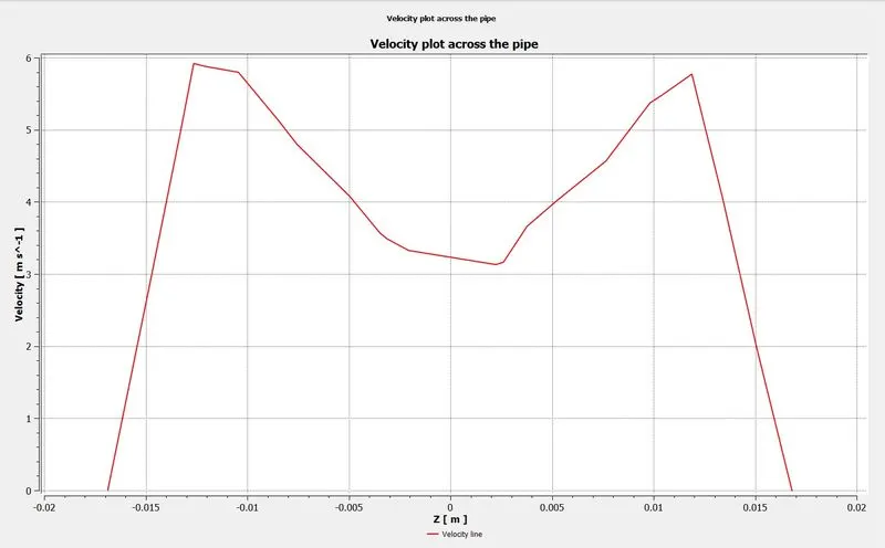
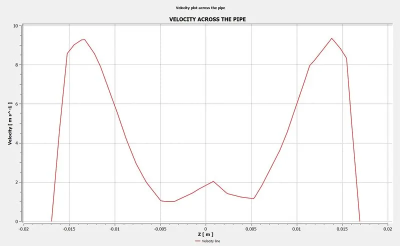
Velocity contour and respective plot across the pipe:
Study 2: (Case 1 ---> K-Omega model)
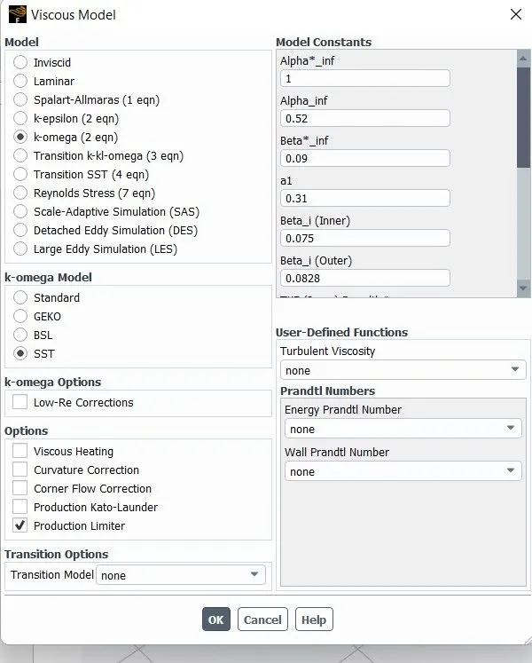
Parameters taken in study 2:
Model : K-Omega Model, SST
Solver : Pressure-Based
Velocity formulation : Absolute
Time : Steady
Meshing : Automatically generated.
Considered the Energy model.
Input information for the study II:
Velocity at hot inlet - 3 m/s; Temperature at hot inlet - 36 C
Momentum ratio - 2
Velocity at cold inlet - 6 m/s; Temperature at cold inlet - 19 C
The information provided in the study II is quite similar inorder to match the results with the K-Epsilon model and to get the better results comparision.
And also we are choosing the same meshing parameter.
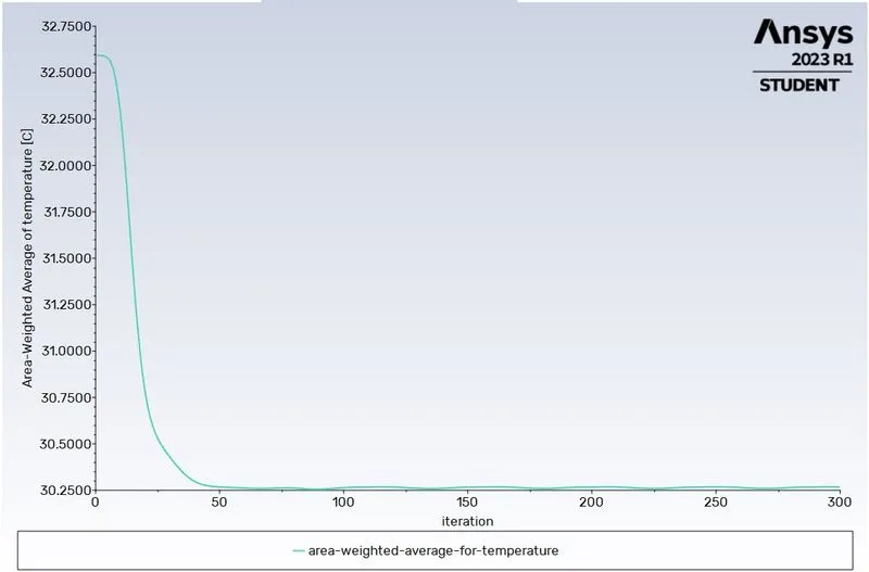
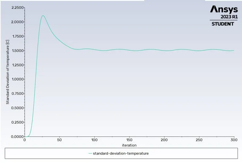
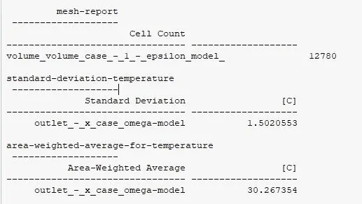
Results Plot:
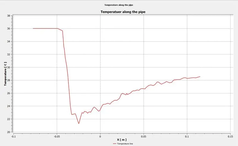
TEMPERATURE CONTOUR AND RESPECTIVE PLOT ALONG THE PIPE:
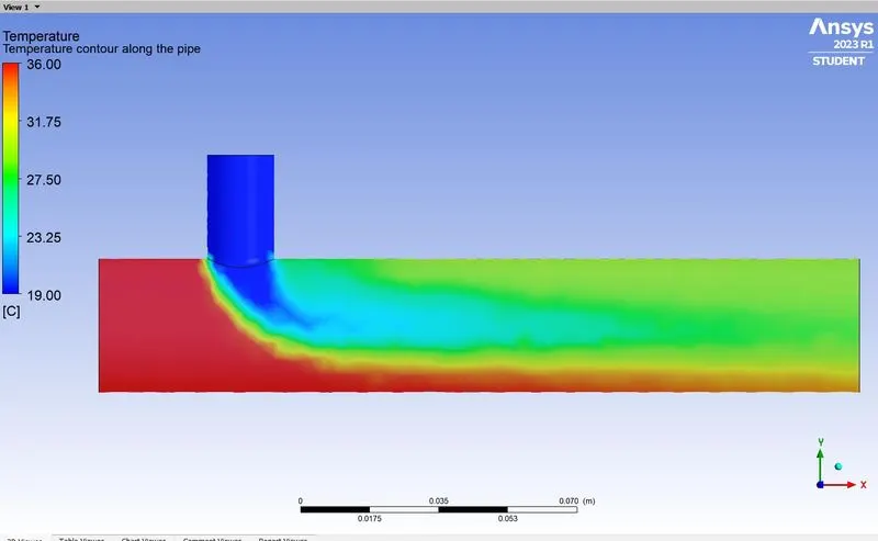
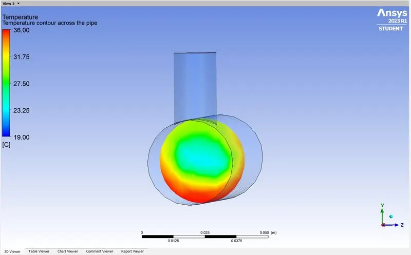
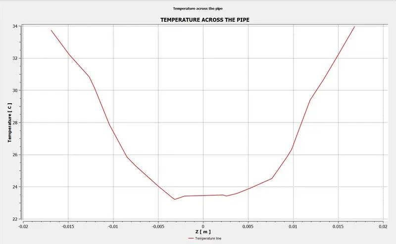
TEMPERATURE CONTOUR AND RESPECTIVE PLOT ACROSS THE PIPE:
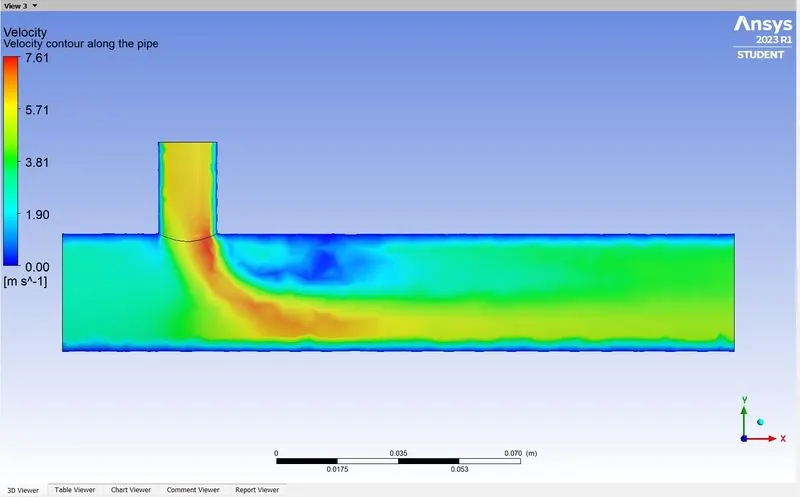
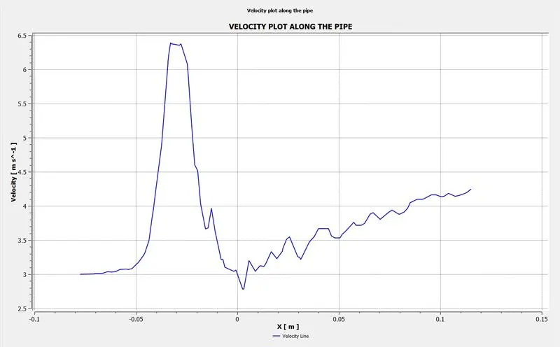
VELOCITY CONTOUR AND RESPECTIVE PLOT ALONG THE PIPE:
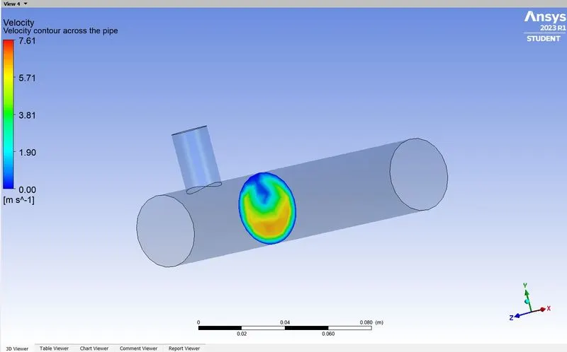
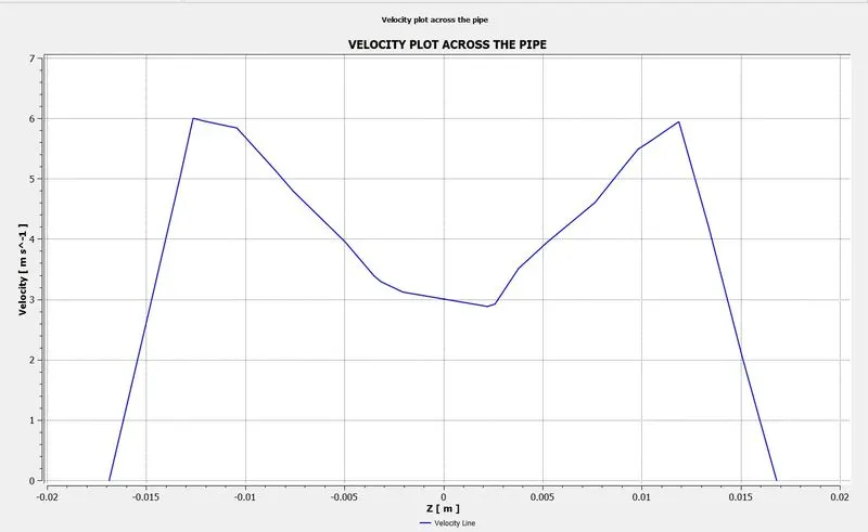
VELOCITY CONTOUR AND RESPECTIVE PLOT ACROSS THE PIPE:
OUTCOME FROM STUDY I AND II:
| STUDY I (K-epsilon) | STUDY II (K-Omega) | |
| Mesh Count | 12780 | 12780 |
| Area-Weighted Average | 30.216648 | 30.267354 |
| Standard Deviation | 1.5749106 | 1.5020553 |
For our geometry considerably both the model's solution are moreover giving the same results. But considering our solution as a low reynold's number model we can preferably go for the K-Omega model for our further calculation. So as of now Case 1 study is done for the momentum ratio 2. We have to produce the results for the momemtum ration 4 and then we can go for the case 2.
Case I - K-0mega Model: Momentum ratio 4:
Parameters taken:
Model : K-Omega Model, SST
Solver : Pressure-Based
Velocity formulation : Absolute
Time : Steady
Considered the Energy model.
Input information:
Velocity at hot inlet - 3 m/s; Temperature at hot inlet - 36 C
Momentum ratio - 4
Velocity at cold inlet - 12 m/s; Temperature at cold inlet - 19 C
Mesh Parameters:
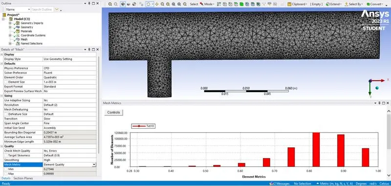
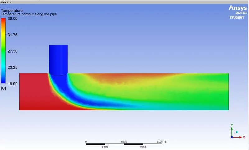
Here I changed the meshing parameters slightly a bit to understand the better flow nearer and over the wall. As we can see in the previous momentum ratio - 2 results. Due to the coarse mesh in and around the wall region, smooth smudging of mix not happened at the flow field. This is due to the fact that while the solving the model from each of the neighbouring nodes, when the element size is high it may not be able to capture the approximation of the two nodes. So by reducing element size and maintaining the nodes to be finer, we can able to do the approximation of the two nearer nodes and the proper mixing of the field occurs.
Element order - Quadratic
Element Size - 0.001mm
Smoothening of mesh - High
Use adaptive sizing - Yes
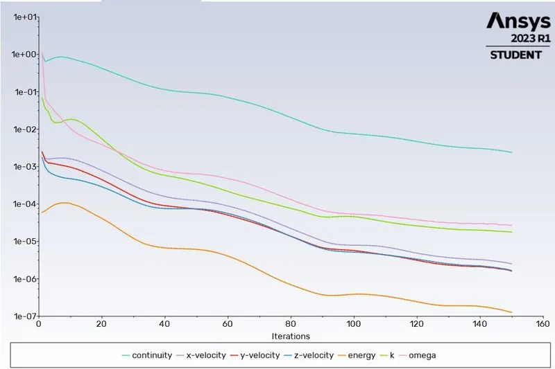
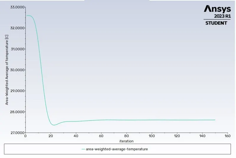
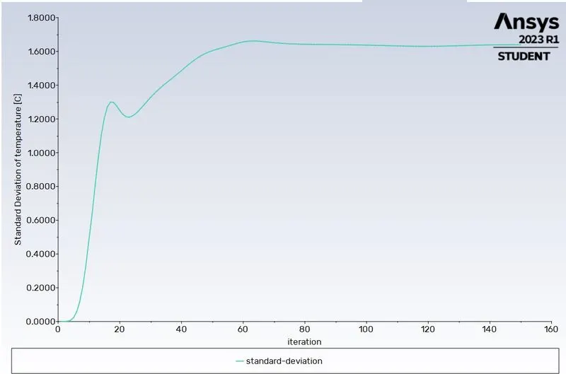
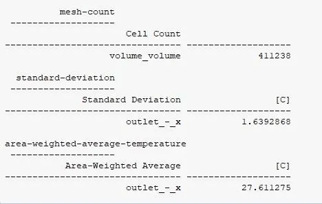
Results Plot:
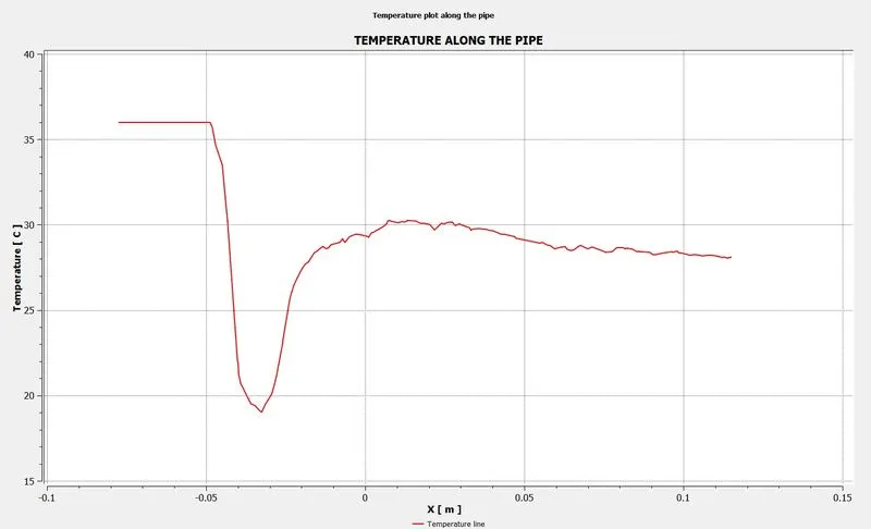
TEMPERATURE CONTOUR AND RESPECTIVE PLOT ALONG THE PIPE:
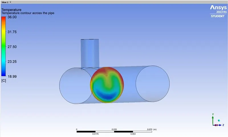
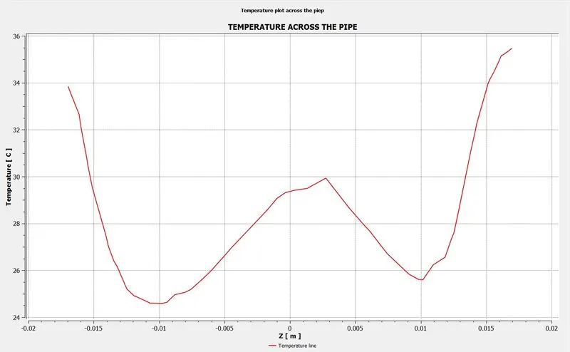
TEMPERATURE CONTOUR AND RESPECTIVE PLOT ACROSS THE PIPE:
VELOCITY CONTOUR AND RESPECTIVE PLOT ALONG THE PIPE:
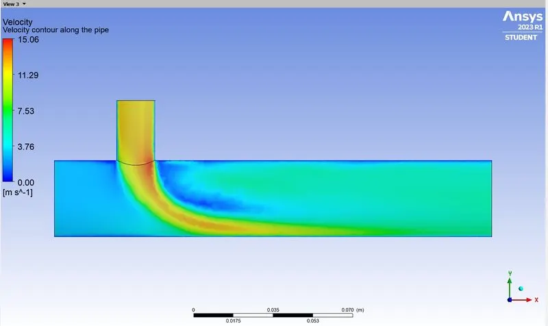
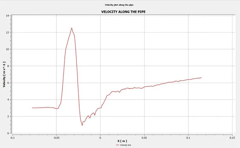
VELOCITY CONTOUR AND RESPECTIVE PLOT ACROSS THE PIPE:
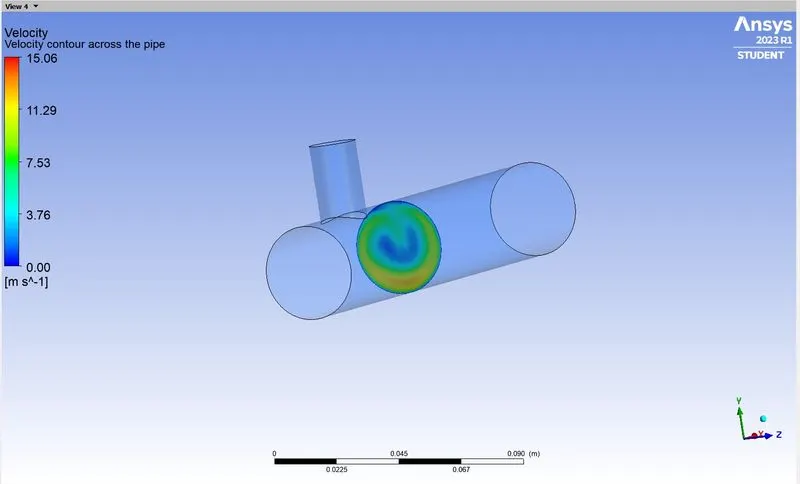
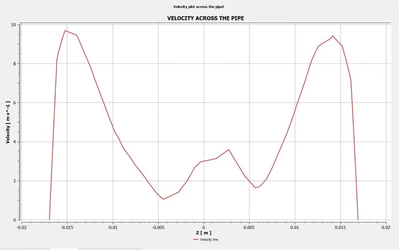
Case II - K-0mega Model: Momentum ratio 2:
Parameters taken:
Model : K-Omega Model, SST
Solver : Pressure-Based
Velocity formulation : Absolute
Time : Steady
Meshing : Automatically generated.
Considered the Energy model.
Input information:
Velocity at hot inlet - 3 m/s; Temperature at hot inlet - 36 C
Momentum ratio - 2
Velocity at cold inlet - 6 m/s; Temperature at cold inlet - 19 C
Mesh Parameters:
Element order - Quadratic
Element Size - 0.001mm
Smoothening of mesh - High
Use adaptive sizing - Yes
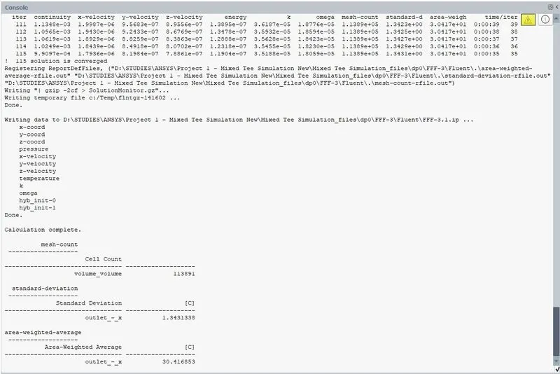
Results Plot:
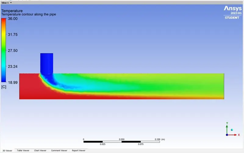
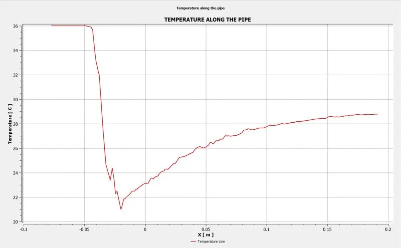
TEMPERATURE CONTOUR AND RESPECTIVE PLOT ALONG THE PIPE:
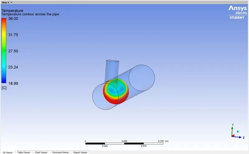
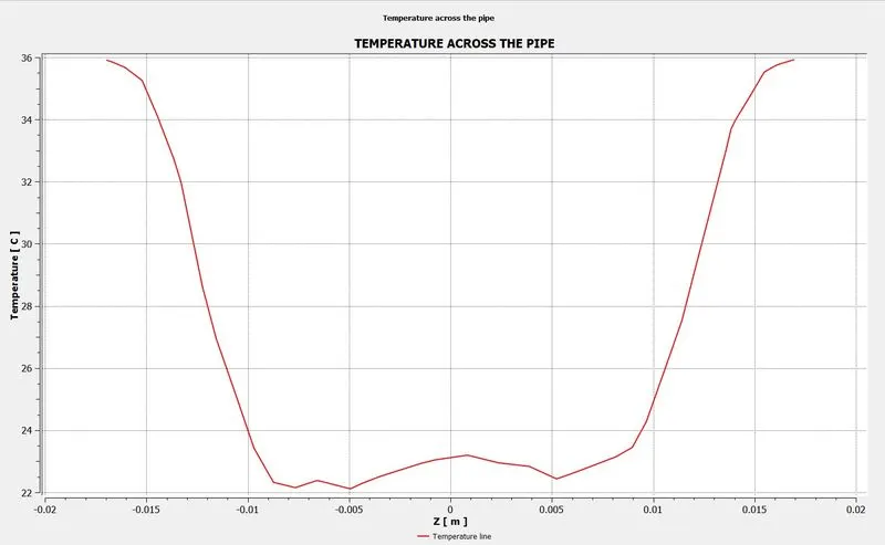
TEMPERATURE CONTOUR AND RESPECTIVE PLOT ACROSS THE PIPE:
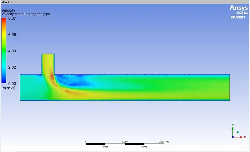
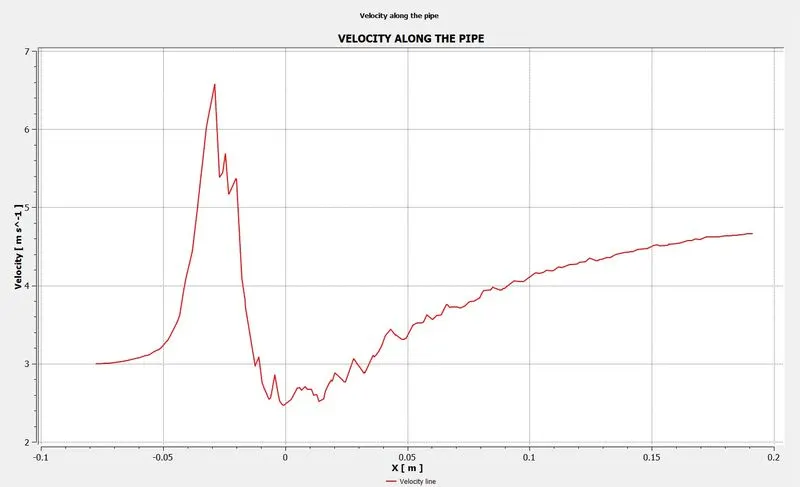
VELOCITY CONTOUR AND RESPECTIVE PLOT ALONG THE PIPE:
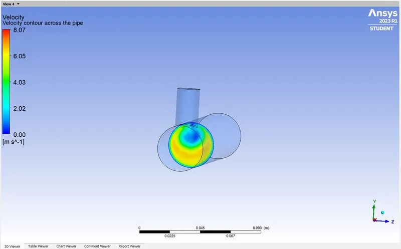
VELOCITY CONTOUR AND RESPECTIVE PLOT ACROSS THE PIPE:
Case II - K-0mega Model: Momentum ratio 4:
Parameters taken:
Model : K-Omega Model, SST
Solver : Pressure-Based
Velocity formulation : Absolute
Time : Steady
Meshing : Automatically generated.
Considered the Energy model.
Input information:
Velocity at hot inlet - 3 m/s; Temperature at hot inlet - 36 C
Momentum ratio - 4
Velocity at cold inlet - 12 m/s; Temperature at cold inlet - 19 C
Mesh Parameters:
Element order - Quadratic
Element Size - 0.001mm
Smoothening of mesh - High
Use adaptive sizing - Yes
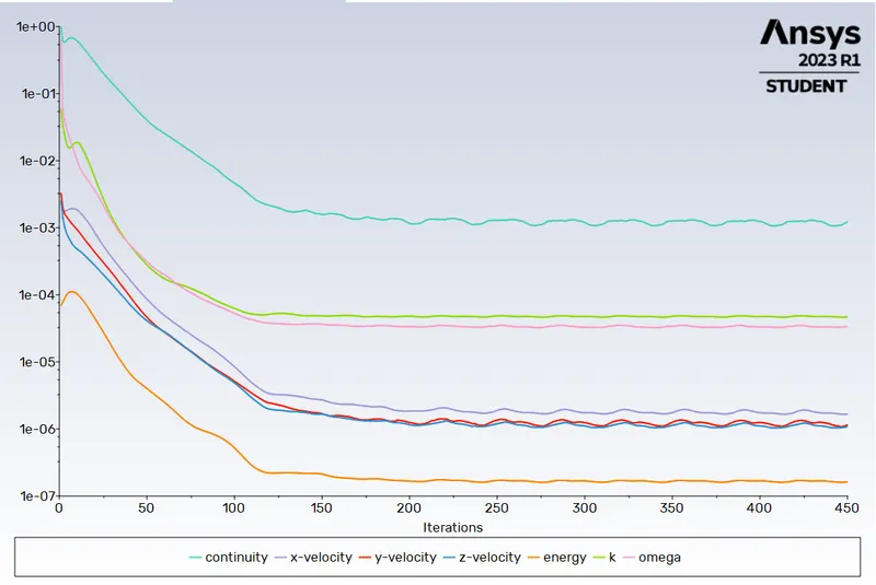
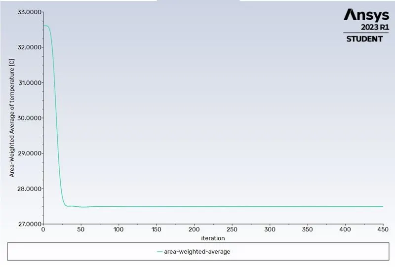
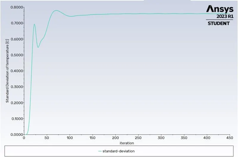
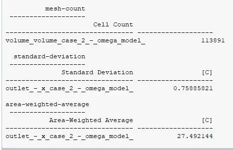
Results Plot:
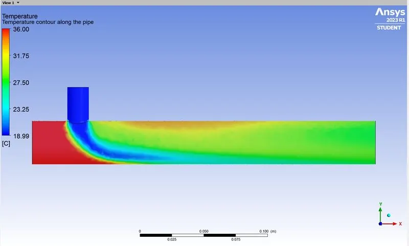
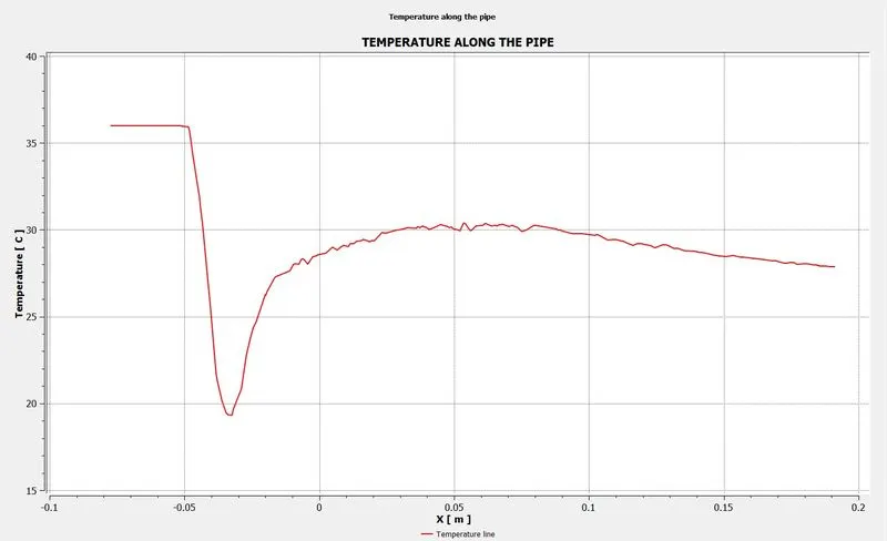
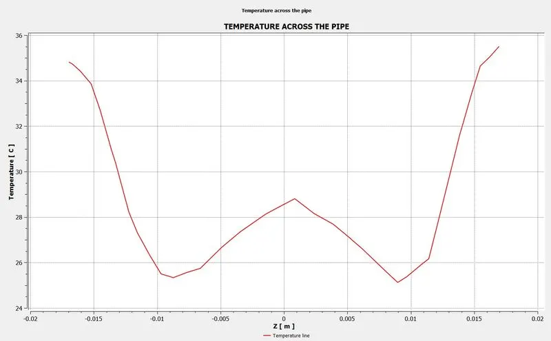
TEMPERATURE CONTOUR AND RESPECTIVE PLOT ALONG THE PIPE:
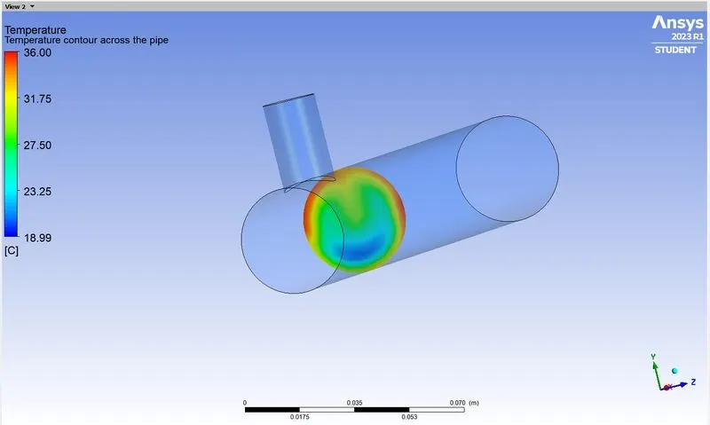
TEMPERATURE CONTOUR AND RESPECTIVE PLOT ACROSS THE PIPE:
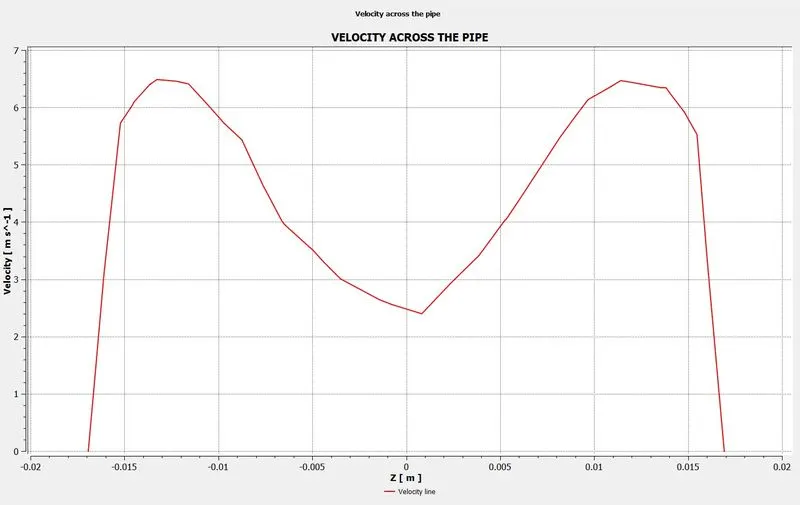
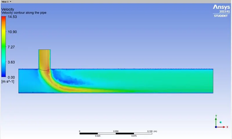
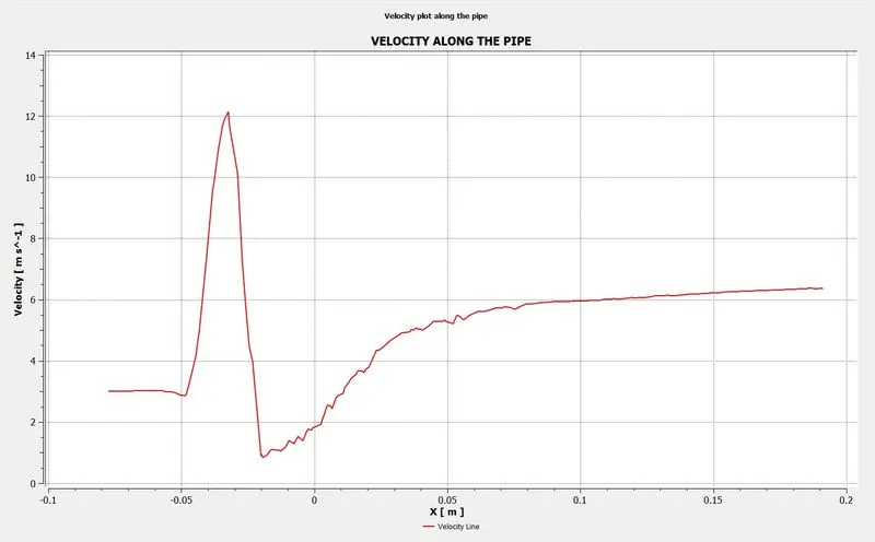
VELOCITY CONTOUR AND RESPECTIVE PLOT ALONG THE PIPE:
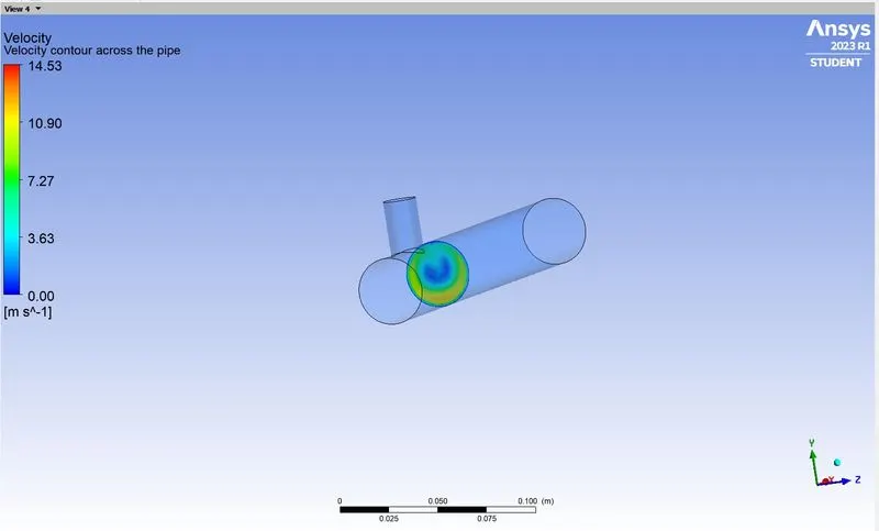
VELOCITY CONTOUR AND RESPECTIVE PLOT ACROSS THE PIPE:
FINAL RESULTS:
Effect of Moment Ratio :
| Case II - K-0mega Model | |
| Moment Ratio - 2 | Moment Ratio - 4 |
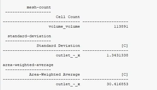
By observing the Case II, with the same properties, models and parameters we can able to see that moment ratio -4 increases fine mixing of the fluid at the end of the outlet as the standard deviation range decreases comparing the moment ratio 2. And also the temperature is also reduced in the moment ratio -4 indicates the well mixing of the fluid inside the flow. And by viewing the velocity plot along the pipe for the two cases,
Effect of Length:
| Case II - K-0mega Model - Moment Ratio 2 | |
| Short Tee | Long Tee |
By observing the velocity plot, there is a slight increase in velocity profile in the Long tee than the short tee at the outlet. And also the mixing of the fluid is quite good while looking up on the standard deviation results for Long tee than the short tee. So by the increase in the length the effective mixing happens.
LEARNING OUTCOMES:
By performing this simulation study we can able to get the insight of
- How the mixing tee works
- How the length and moment ratio affects the effective mixing.
- Proper meshing for obtaining accurate results.
- Variation of models affect mixing of fluid.