Week 1- Mixing Tee

Aim :-

Solve the mixing of hot and cold fluid diffusion for a given problem using work bench and fluent under steady-state simulations and compare the mixing effectiveness when hot inlet temperature is 36°C & the Cold inlet is at 19°C. Use the k-omega SST model for all cases.

Case 1: Short mixing tee with a hot inlet velocity of 3 m/s and Momentum ratio of 2 & 4.

Case 2: Long mixing tee with a hot inlet velocity of 3 m/s and Momentum ratio of 2 & 4.

In a table, compare the following values from the 2 cases.

• Cell count
• Average outlet temperature (Theoretical & Numerical)
• Number of iterations for convergence

INTRODUCTION :-

Mixing Tee are a pipe joint in form of T-joints in which two fluid streams with different physical and/or chemical properties mix These are widely used in the petrochemical industry and also used in HVAC Industries.

THEORY :-

Mixing Tee, The term TEE denotes the joint at a 90°, where the energy losses will be more as compared to smooth bends. So this problem is majorly seen while designing ducts for air conditioning. The conditioned air around 30-50% is mixed with the fresh air , the mixing percentage depends on what temperatre we want to achieve at the outlet. In summers the mixing percentage of the condenced air is more and for winter the mixing percentage of condenced air is low. it depends that we are using the duct for only as a air conditioner or a blower. After mixing the two airs at different velocity and temperature the air is recirculated to the room space before conditioning it to the human comfort level. This help in increasing the quality of the air.

Main objective of this problem is to plot the temperature and velocity profile of the fluid with respect to the length of the pipe and to study the temperature at oulet fluid which is mixed on the ANSYS FLUENT to compare the results with numerical equations.

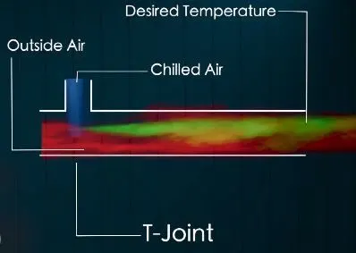
The problem corresponds to a control volume across which mass flow takes place with a mixing of same fluid from two inlets at different velocities and temperatures.

In order to solve for the velocity at outlet, the law of conservation of mass can be used;

Assumptions: Fluid is incompressible, velocity is constant throughout the cross- section, and

Steady-state (Given)

ʃ_cs Ƥ V. dA = 0 ………………..(1)

Where, Ƥ = density of air

V.dA = dot product of velocity vector(V) and area vector of a small area element dA.

The control surface is the boundary of the control volume surrounding the mixing tee. For convenience, it can be considered to be a rectangle encasing the entire model with inlets and outlet at 90 degrees to the flow direction.

Since, there are two inlets and one outlet, we can write equation (1) as;

ʃ_cs Ƥ V. dA = ʃ_Ah Ƥ V_Ih. dA + ʃ_Ac Ƥ V_Ic. dA + ʃ_Ao Ƥ V_O. dA = 0

Rate of mass flux Rate of mass flux Rate of mass flux

through hot inlet through cold inlet through outlet

The density of the air is assumed to be constant, so upon simplifying the above equation,’

We get,

……………………. (2)

For getting the temperature at outlet, let`s use the steady state energy balance equation from first law of thermodynamics:

dE_cv / dt = Q^._cv - W^._cv + Σ m^._I ( h_I + V_I²/2 + gz_i ) - Σ m^._e ( h_e + V_e²/2 + gz_e ) = 0

Assumptions: 1. Changes in K.E and P.E are negligible

2. No heat transfer across the walls

In addition, since there is no work done on or by the system, the equation gets reduced to;

Σ m^._I h_I = Σ m^._e h_e ……………….. (3)

In our case, since we have two inlets and one outlet, equation (3) can be re-written as;

m^._Ihh_Ih + m^._Ich_Ic = m^._oh^._o

Enthalpy of Enthalpy of Enthalpy of

Hot inlet air cold inlet air mixed outlet air

Since, h = c_pT, we can simplify the above equation as below;

…………………….. (4)

SOLVING AND MODELLING APRROACH :-

We have two model of Mixing Tee one is Short TEE and other is Long Tee model. The model are made in solidworks and we have the STEP file for importing it into ANSYS Fluent .The hot fluid and cold fluid enters the main pipe and branched pipe respectively. We will use Steady State solver to find out the temperture at the outlet with no heat generation or heat transfer of the Mixing Tee.

we will be using K-epsilon And K-omega to solve this problem for the dollowing two cases :-

Case 1: Short mixing tee with a hot inlet velocity of 3 m/s and Momentum ratio of 2 & 4.

Case 2: Long mixing tee with a hot inlet velocity of 3 m/s and Momentum ratio of 2 & 4.

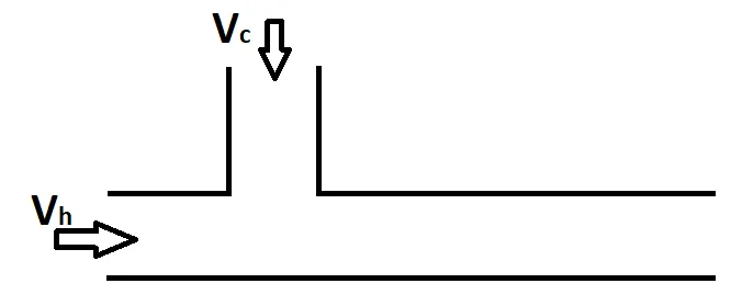
Momentum Ratio is the ratio between the velocity of Cold Fluid and Hot fluid.

Momentum Ratio :- V_c / V_h

where V_c is velocity of Cold fluid entering the pipe.

V_h is velocity of Hot fluid entering the pipe.

PREPROCESSING AND SOLVER SETTING :-

For Analysing the temperature at outlet we need the geometry of the Mixing Tee model

we will import the geometry in Ansys workbench in fluent flow module.

Procedure of importing the file to ANSYS Worknbench in Fluent Flow Module.

1. We will first make a folder in any of the drives named as Mixing TEE and save the downloaded files there.

2. We will then Ansys workbench

3. Open a new fluid flow (Fluent) system.

4. Now we will import geometry in the Fluent system by clicking a right button of mouse on Geometry

Geometry - Import Geometry - Browse - select file - open.

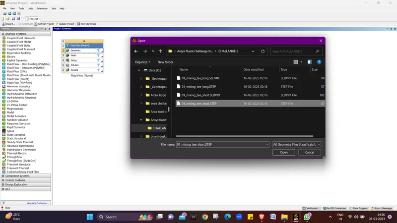
5. We can see the Green tick in the geometry tab that means the geometry is imported successfully and now we will use Edit Geometry in Spaceclaim.

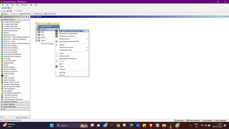
6. we can see the model is imported successfully in spaceclaim.

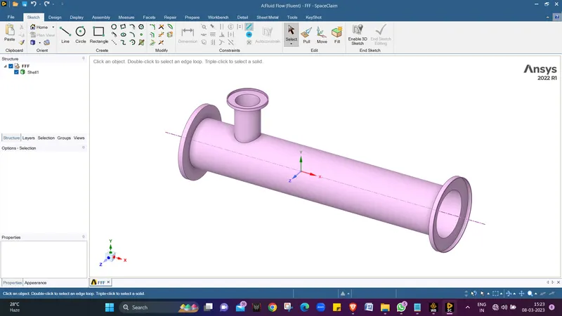
7. we will now go to prepare tab and click on Volume extract tool.

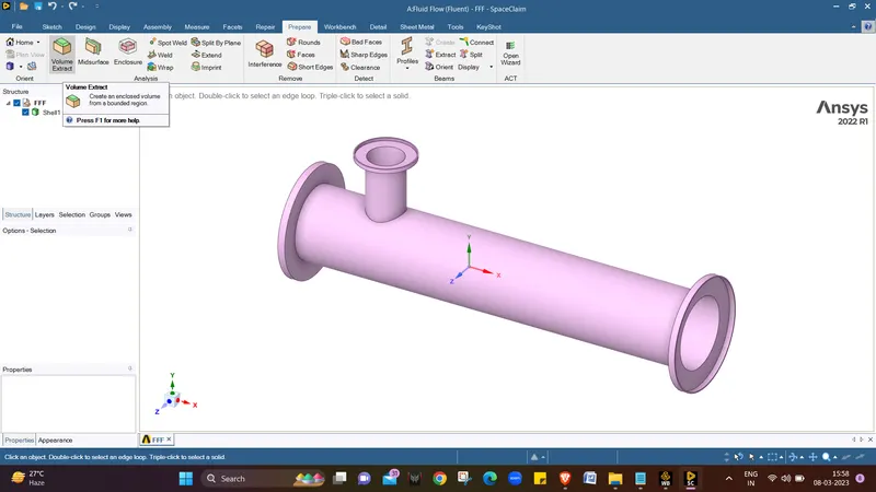
8. Now we will select Edges for selection and activate it by making a left clicjk over it.

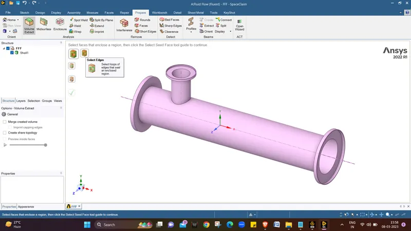
9. As we can see that the selct edges tab is active now.

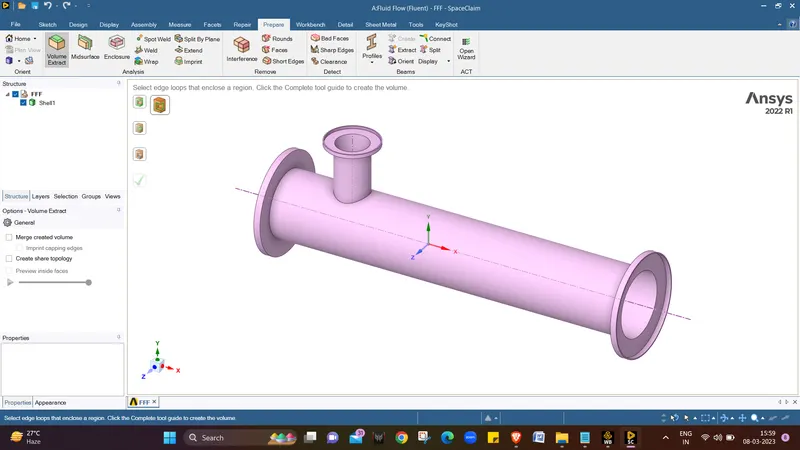
10. now we will select the edges for volume extraction.

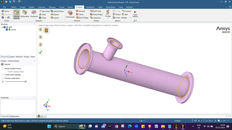
11. Now we will click on the tick to complete the volume extraction.

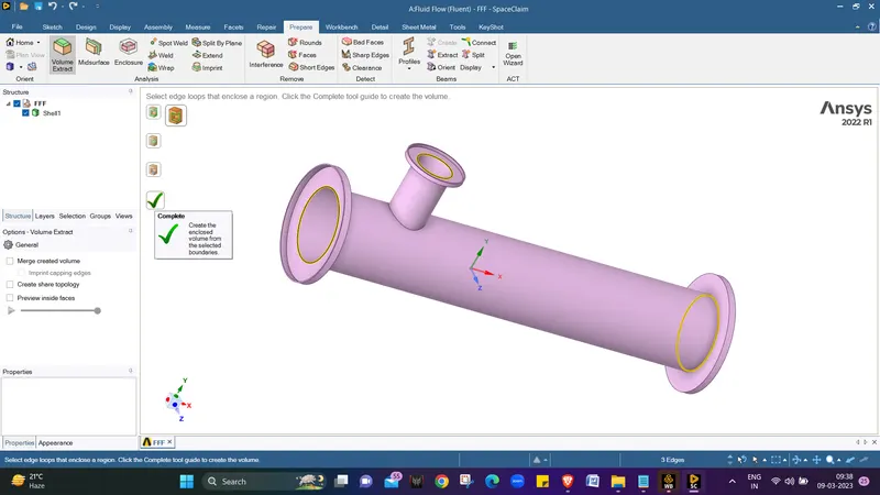
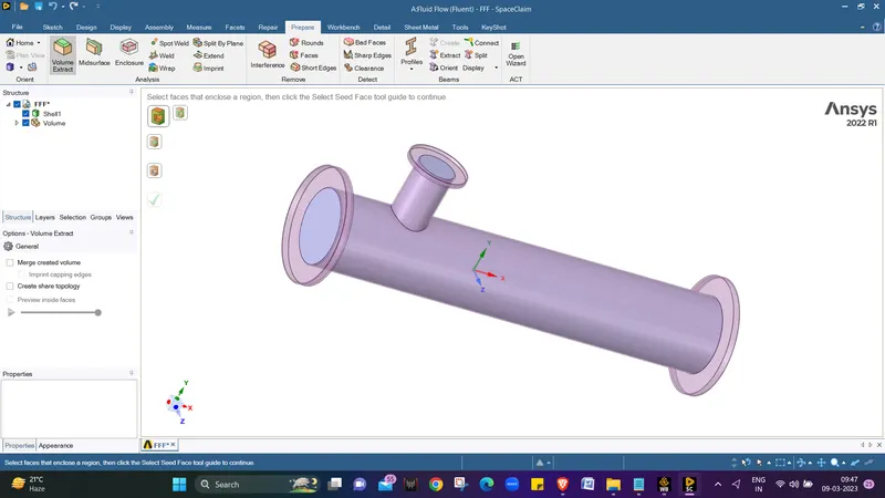
12. Now we can see that the volume has been extracted.

13. Now in the left side column where the shell and volumes are highlighted we will right click on Shell And select "Supress for Physics"

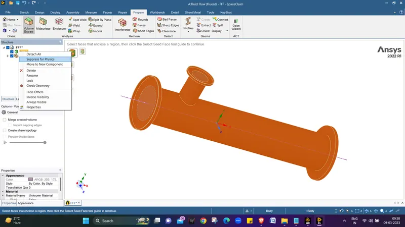
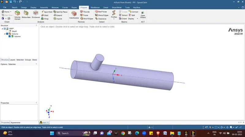
14. We can see the fluid volume is extraxted succesfully.

15. Now we will close the spaceclaim window and move to main project window.

16. Double click on Mesh to open the mesh module.

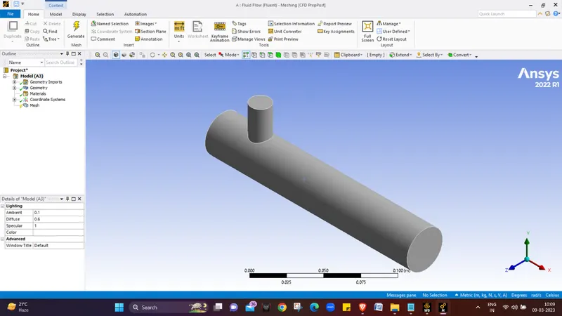
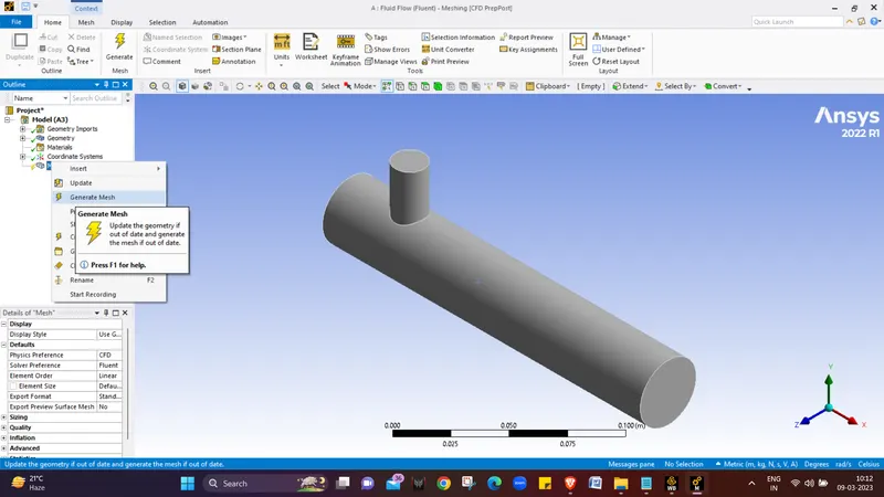
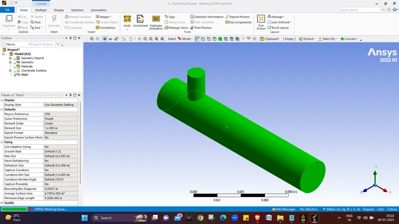
17. we will right click on mesh and select generate mesh or update. this will produce a default mesh by the Ansys fluent mesh module on basis of a CFD.

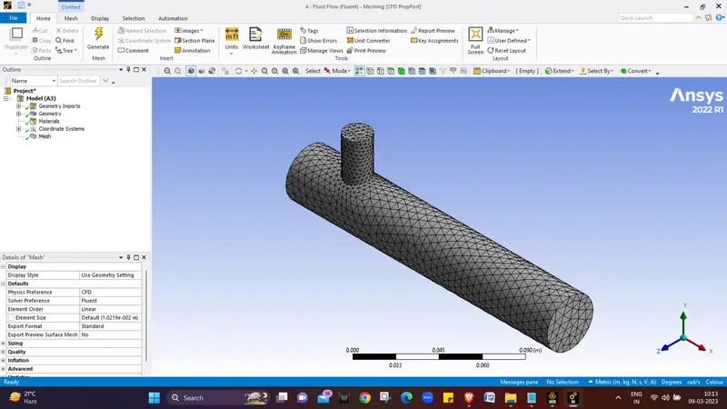
18. We can see that its a course mesh and we are having 12780 elements.

19. We will go for a fine mesh where element size will be 1 mm.

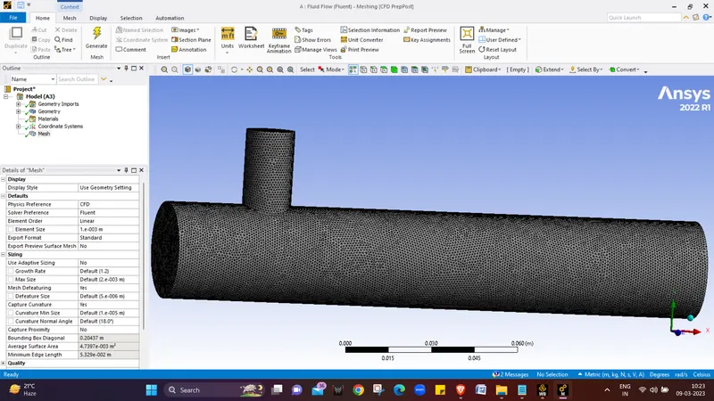
20. We can see that a very fine mesh is produced with element count as 576721.

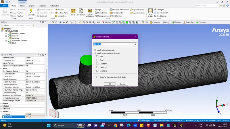
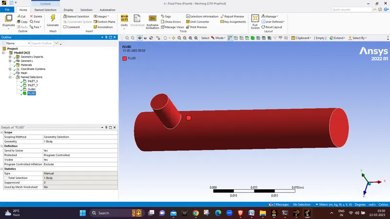
21. Now we will go for named selection, we wil use face selction mode and select a face then right click on it and select "Create Named Selection" ow we can use a shortcut select face and press N on the keybord.

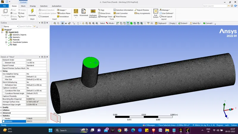
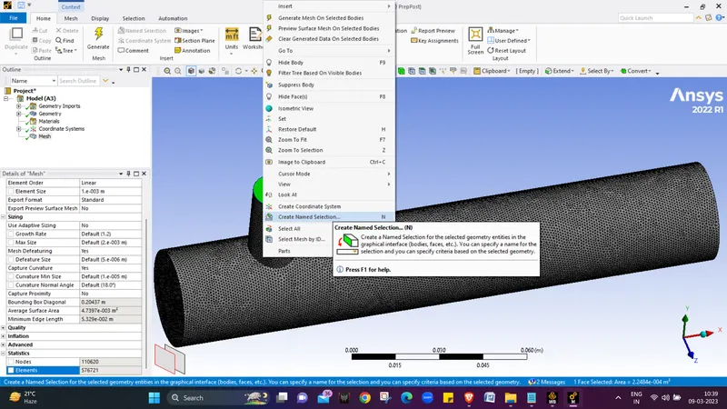
22. A window open in which we will rename the face as INLET_X and click ok.

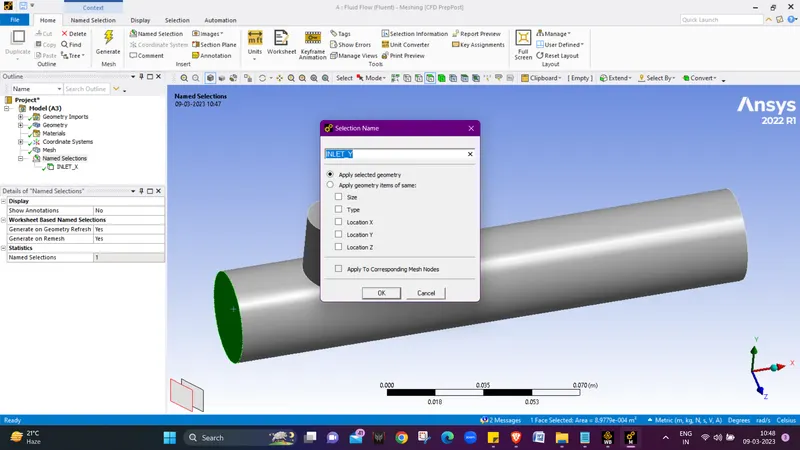
23. Now we will define INLET_Y

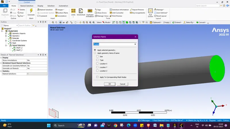
24. Now we will define OUTLET.

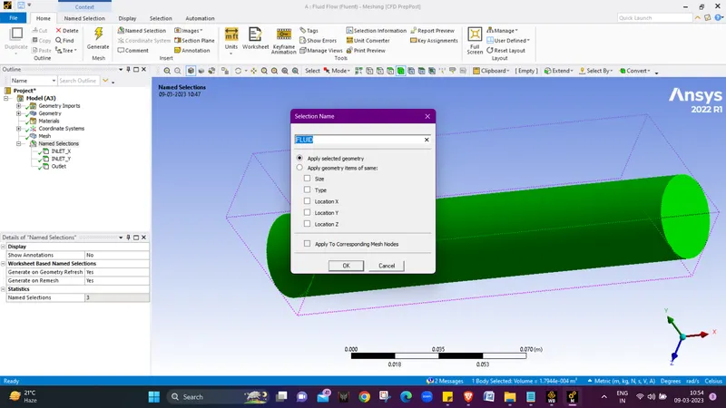
25. We have to also name selection for volume which will be done using Body selection tool. and the volume will be named as FLUID. and with the face selection tool we will define new nam selection as walls.

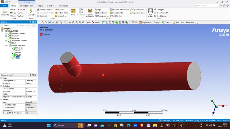
26. Now we will close the window and again go back to the project window and select mesh and right click on it and select update.

Setup :-

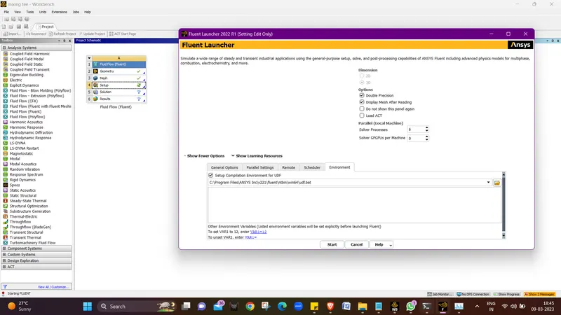
• In order to begin solution setup, go to the Workbench Project page and double click on the setup, make sure double precission is selected and gives number of solver processes as 6 and click on Start for student version the solver processes can't exceed more than 4.
• project - Setup - physics - select steady state - pressure based absolute velocity and enable energy equation since we are going to find the temperature of the fluid.

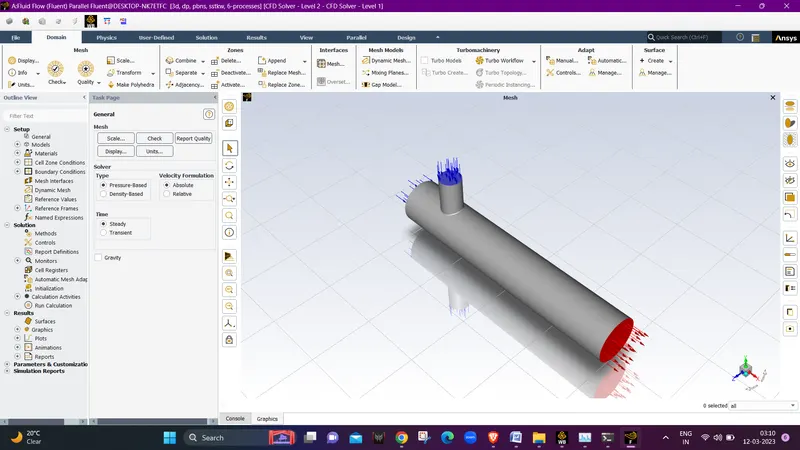
• Now we give the boundary conditions inlet velocity 3 m/s for hot inlet and 6 m/s for the cold inlet also give temperature for cold fluid as 19°C and for hot fluid 36°C.
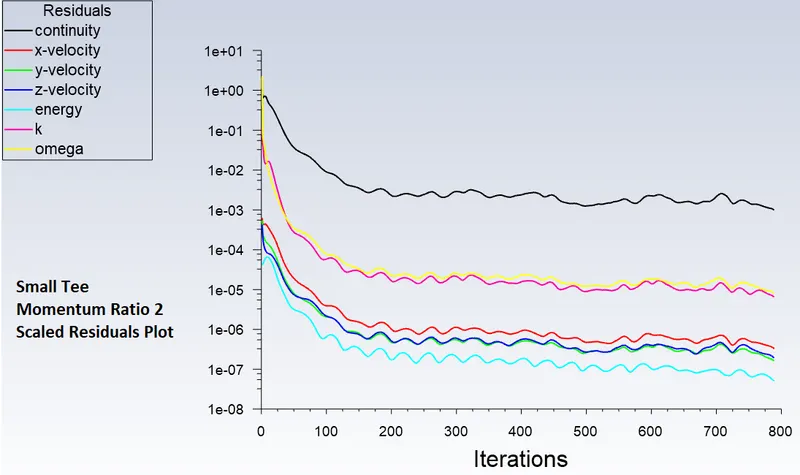
• After performing all these steps we will go to solution tab and we will use hybrid initialization and then we will run the calculation for around 800 time steps till the solution gets converged.

  
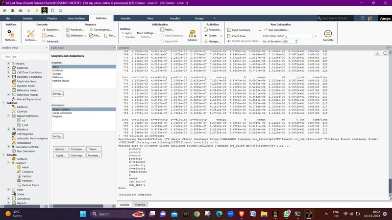
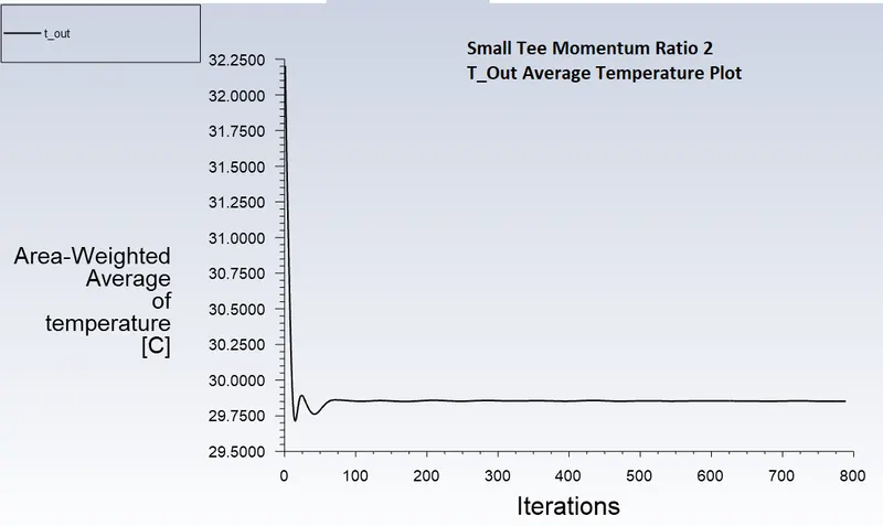
• we can see the solution is converged at 789 iterations .
• Now we will first create a plane in X-Y plane and then we will make contor plots for Temperature, Velocity, Pressure and vector velocity in the Graphics Tab.
• now we will repeat the whole process for other cases too and after that we will compare the results.

Results:

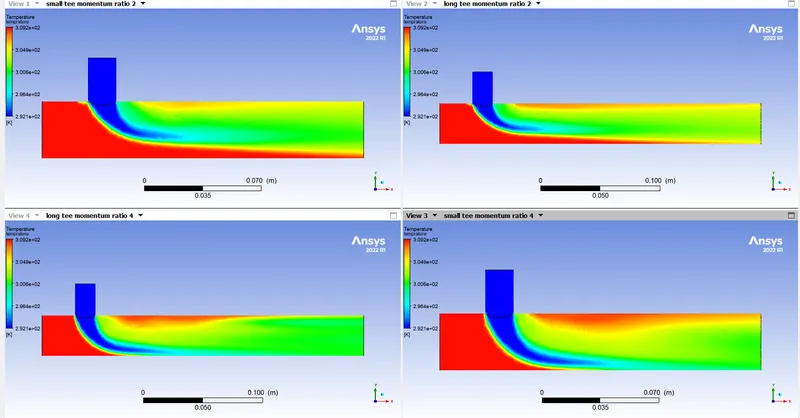
Temperature plot at plane 1 :-

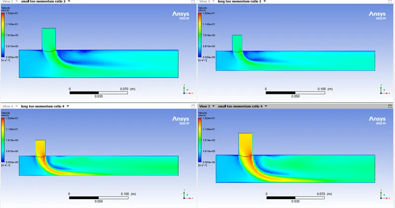
Velocity plot at plane 1:-

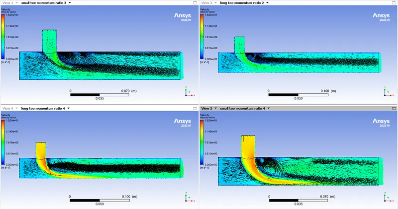
Velocity vector plot at plane 1:-

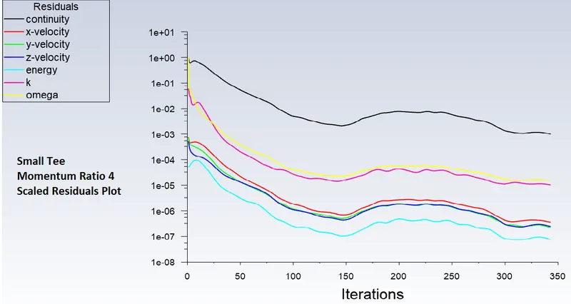
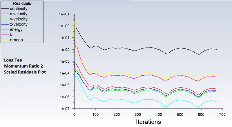
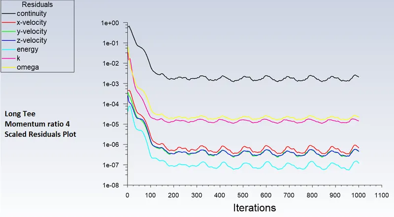
Scaled Residuals PLots

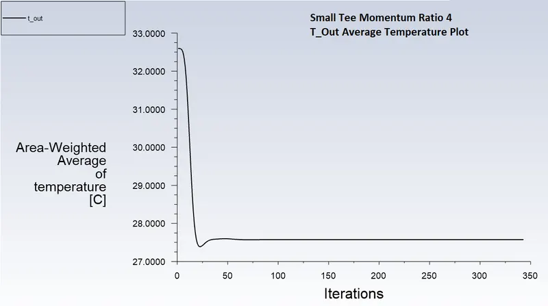
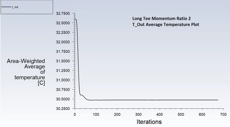
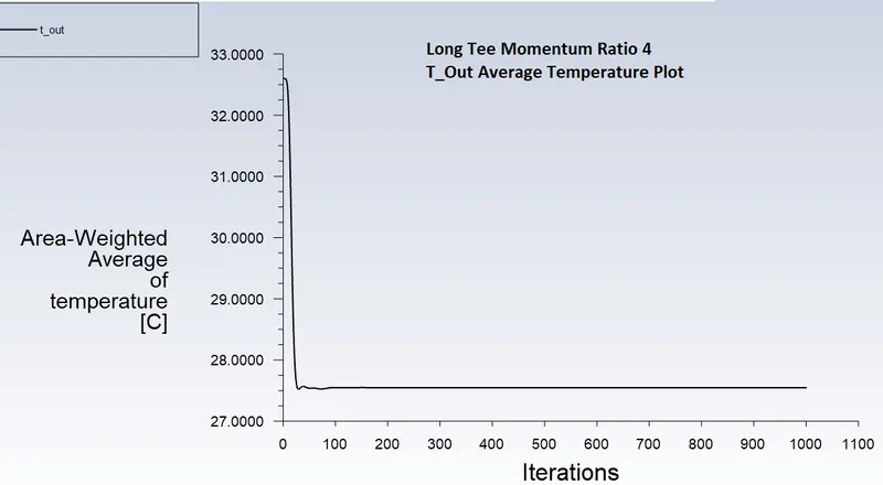
T_out Average Temprature PLots

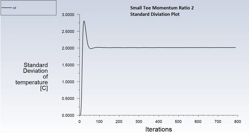
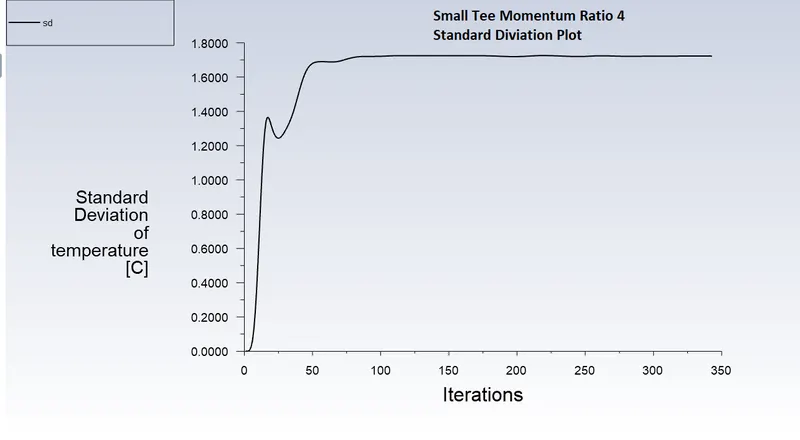
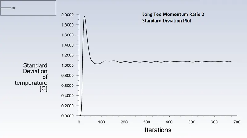
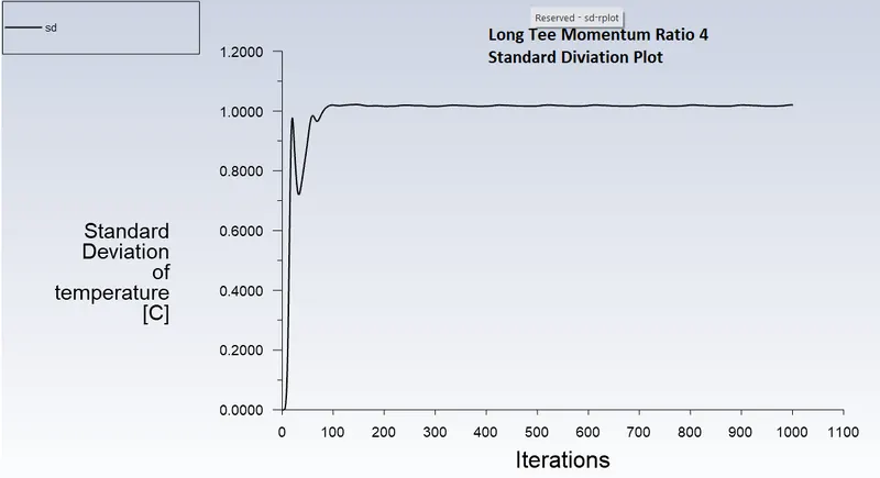
Standard Diviation PLots

Conclusion:

From the perusal of the above results, it can be concluded that:

1. The length of the mixing Tees does not have an appreciable amount of change in the final values of temperature and velocity.
2. The mixing is better with a MR=4 in both short and long Tees as is revealed from the analysis of above results.