Week 1- Mixing Tee

OBJECTIVE:

The objective of this project is to set up steady-state simulations to compare the mixing effectiveness when hot inlet temperature is 36⁰C & the Cold inlet is at 19⁰C in a mixing tee model of varying lengths and to understand the effects caused on the liquid due to the varying lenghts of the pipes.

→ Case-1:

• Short mixing tee with a hot inlet velocity of 3m/s.
• Momentum ratio of 2 & 4.

→ Case-2:

• Long mixing tee with a hot inlet velocity of 3m/s.
• Momentum ratio of 2 & 4.

PROCEDURE:

1:Pre Processing:

1. Workbench→under Analysis sysmtem select Fluid flow(fluent) drag and drop it in Priject schematic → Geometry → New spaceclaim geometry.
2. Spaceclaim for geometry cleaning→ File select the appropiriate file and the Open.
3. Prepare → for selecting the fluid flow path → Edge selection select the required edges the click the tick option.
4. To show only the selested fluid path volume under Structures unselect the soild part, since we going to study only the fluid flow in this project we can disable the soild part Structure → Solid 1 → Supress for physics.
5. Then we can close the spaceclan window the processed geometry will be saved automatically.

Given CADD model:

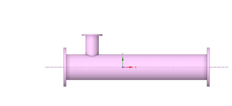
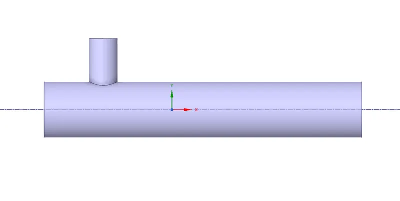
2:Meshing:

1. To generate mesh Workbench → Project schematic → Mesh right click Edit.
2. For defining the mesh target length Mesh→ Details of the "Mesh" → Mesh Metric → Element size we are using a 3mm target lenght mesh.
3. Then to generate mesh Mesh right click Generate Mesh.
4. Details of "Mesh" → Mesh Metric →Element Quality then histogram will appear shoing the quality of the mesh.
5. Then naming the Parts like inlet and out, first select the part and then give the names respectively.
6. shortcut key for face selection CTRL+F and give name press (N) for naming the faces like inlet,outlet,walls show in fig below

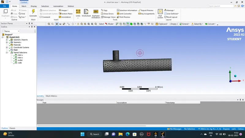
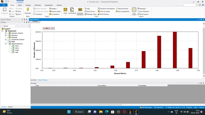
3:Solving:

1. Workbench → Project schematic → Setup → Physics here we are solving for temperature so we have to enable Energy option then the solver K-epsilon → then we have to define the boundary conditions like inlet and outlet temperature and velocity → Zones Boundaries define the boundary conditions.
2. Then we have to define the required outpets in our case Solution → Reports → Definitions → New → Surface report →Area Weighted Temperature (the average temperature at the output) and Standard deviation.
3. Then we have to initialise the process to set the assigned boundary conditions, then we have to define the No of Iterations and then click Calculate to strat the process.
4. Then we can close the soltuion window the processed solution will be saved automatically.

4:Post processing :

1. In the post processing Results window we can get the desiered results like temperaure and velocity contour plots, temperature and velocity reults in a chart form and we can compare the obtained results.

SOLUTION:

Case 1:

1:Short tee momentum ration=2:

SETUP	K-epsilon
Solver Type	Pressure Based
Velocity Formulation	Absolute
Time	Steady
Viscous Model	Realizable k-epsilon with standard wall function
Material	Fluid type: Air
Cell zones Volume_volume	Fluid type: Air
Boundaries	Inlet x (velocity inlet) Velocity Magnitude 3m/s Temperature – 36 degrees c. Inlet y (velocity inlet) Velocity Magnitude 6m/s Temperature – 19 degrees c. Outlet x (Pressure outlet) Gauge Pressure – 0 pas. Walls – Stationary walls

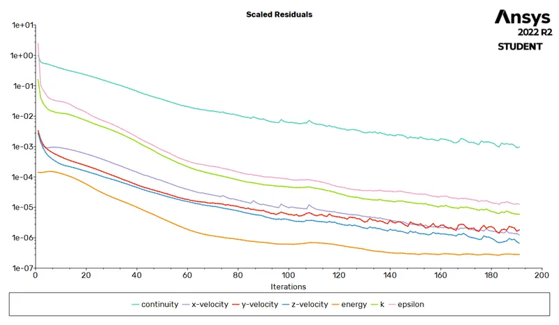
• Residual Plot:

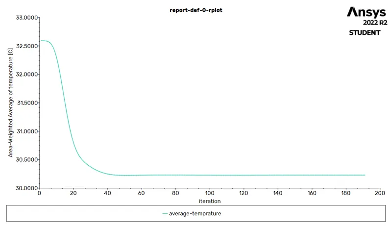
• Average weighted temperature

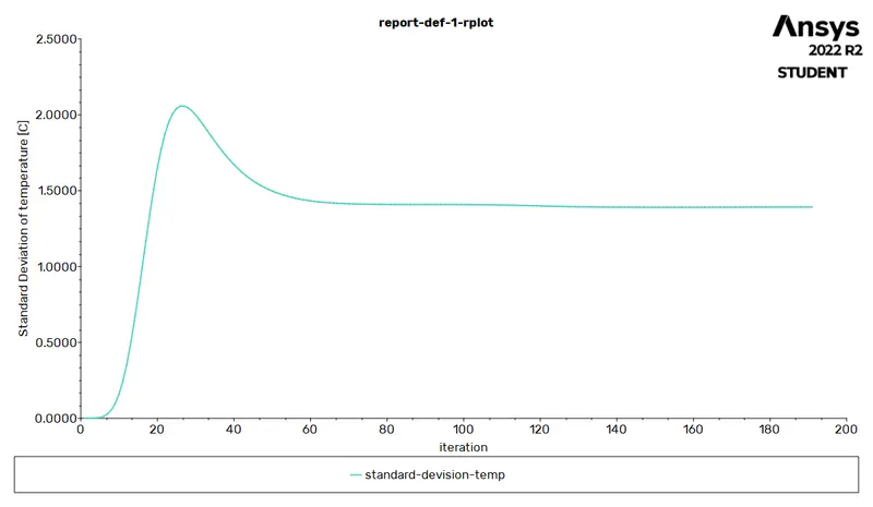
• Standard Deviation

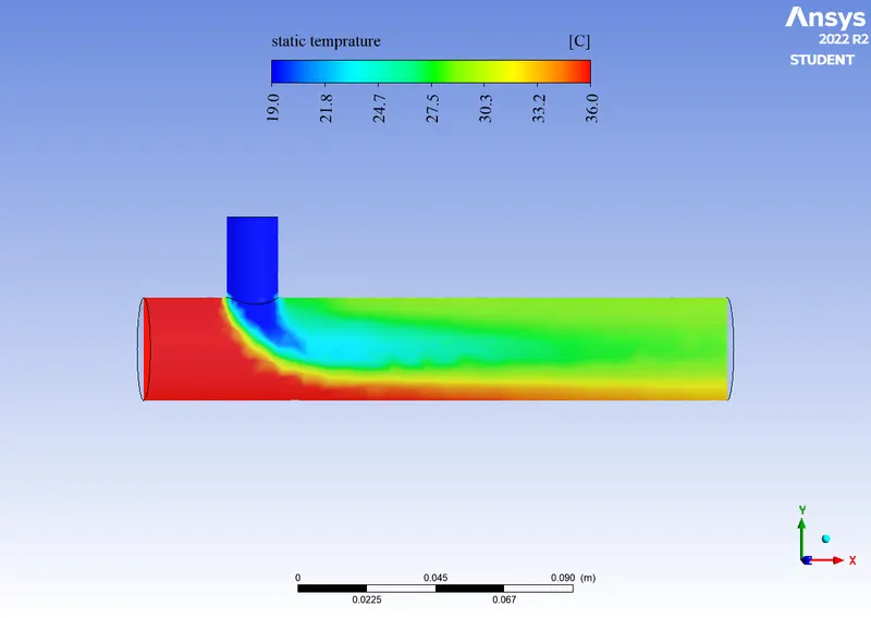
• Temperature contour

• Velocity contour

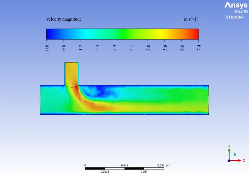
• Velocity vector

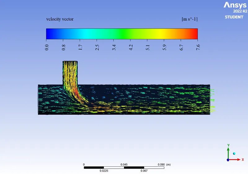
2:Short tee Momentum Ratio=4:

SETUP	K-epsilon
Solver Type	Pressure Based
Velocity Formulation	Absolute
Time	Steady
Viscous Model	Realizable k-epsilon with standard wall function
Material	Fluid type: Air
Cell zones Volume_volume	Fluid type: Air
Boundaries	Inlet x (velocity inlet) Velocity Magnitude 3m/s Temperature – 36 degrees c. Inlet y (velocity inlet) Velocity Magnitude 12m/s Temperature – 19 degrees c. Outlet x (Pressure outlet) Gauge Pressure – 0 pas. Walls – Stationary walls

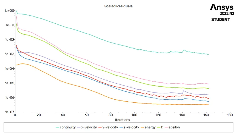
• Residual

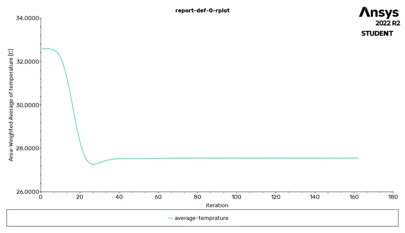
• Average weighted temperature

• Standard Deviation

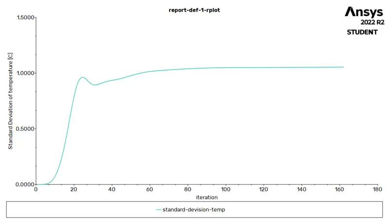
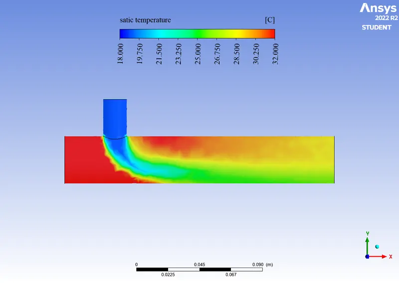
• Temperature contour

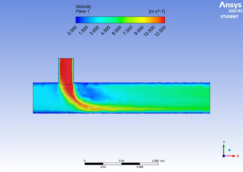
• velocity contour

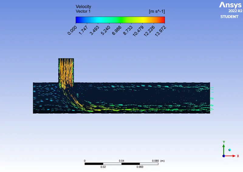
• Velocity vector

• Comparison

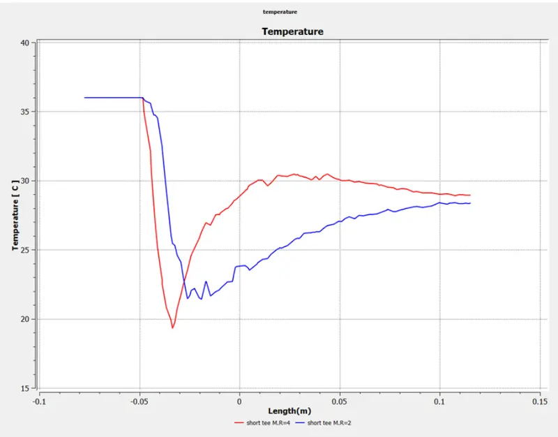
1. SHORT TEE TEMPERATURE:

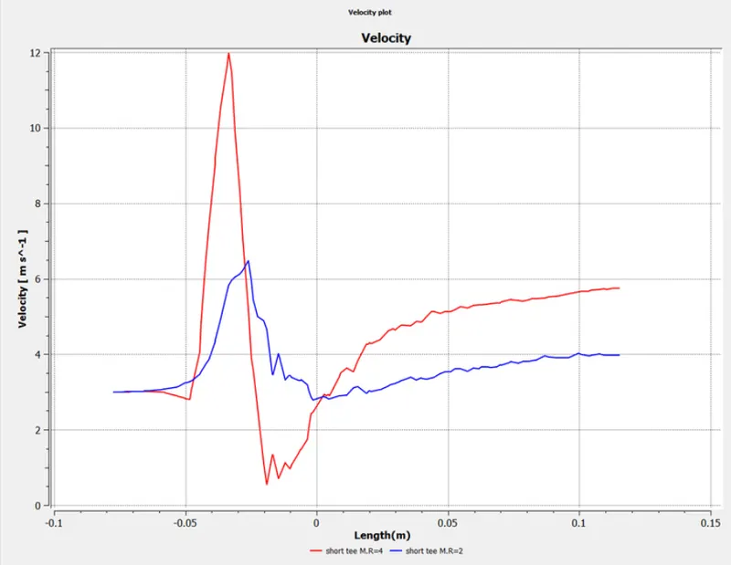
2. SHORT TEE VELOCITY:

CASE 2:

1.Long tee Momentum ratio=2

SETUP	K-epsilon
Solver Type	Pressure Based
Velocity Formulation	Absolute
Time	Steady
Viscous Model	Realizable k-epsilon with standard wall function
Material	Fluid type: Air
Cell zones Volume_volume	Fluid type: Air
Boundaries	Inlet x (velocity inlet) Velocity Magnitude 3m/s Temperature – 36 degrees c. Inlet y (velocity inlet) Velocity Magnitude 6m/s Temperature – 19 degrees c. Outlet x (Pressure outlet) Gauge Pressure – 0 pas. Walls – Stationary walls

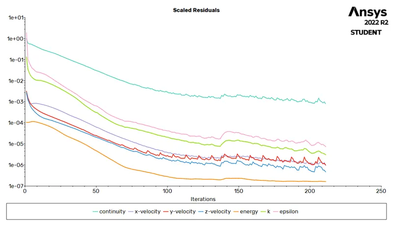
• Residual

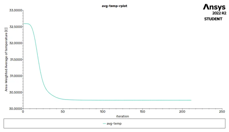
• Average weighted Tempreture

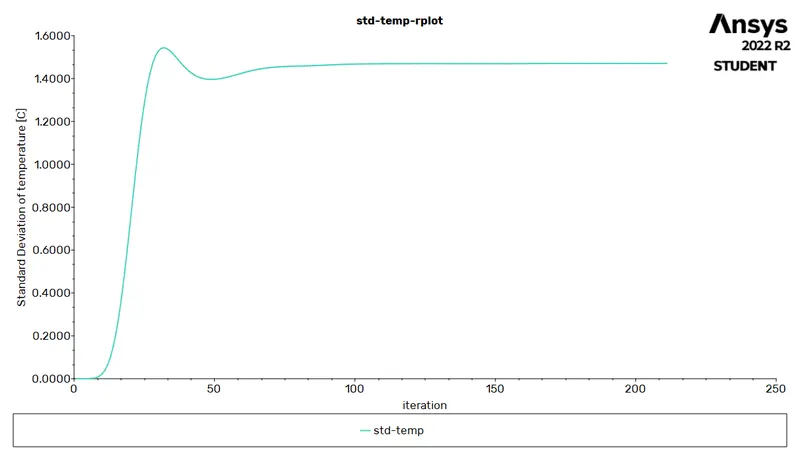
• Standard Deviation

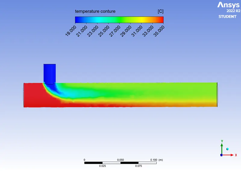
• Temperature contour

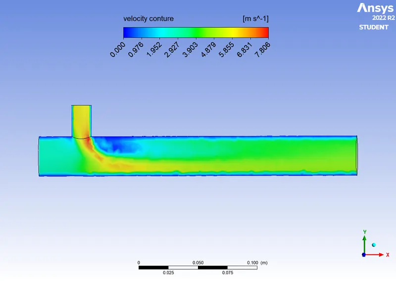
• Velocity contour

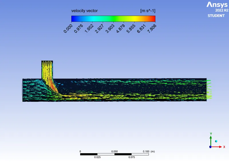
• Velocity vector

2. LONG TEE MOMENTUM RATIO=4

SETUP	K-epsilon
Solver Type	Pressure Based
Velocity Formulation	Absolute
Time	Steady
Viscous Model	Realizable k-epsilon with standard wall function
Material	Fluid type: Air
Cell zones Volume_volume	Fluid type: Air
Boundaries	Inlet x (velocity inlet) Velocity Magnitude 3m/s Temperature – 36 degrees c. Inlet y (velocity inlet) Velocity Magnitude 12m/s Temperature – 19 degrees c. Outlet x (Pressure outlet) Gauge Pressure – 0 pas. Walls – Stationary walls

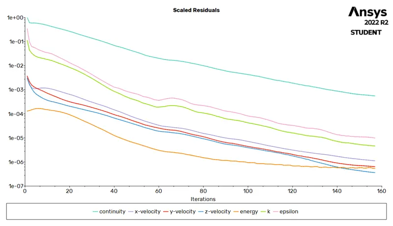
• Residual

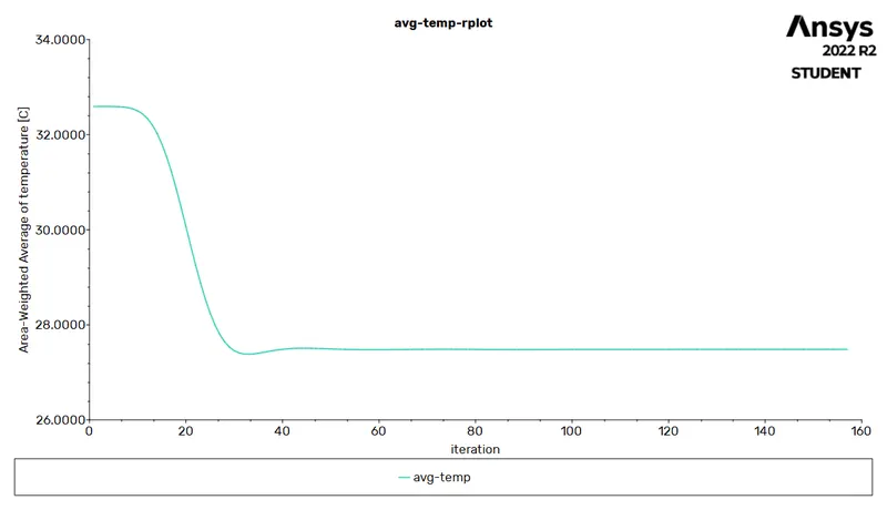
• Average Weighted Temperature

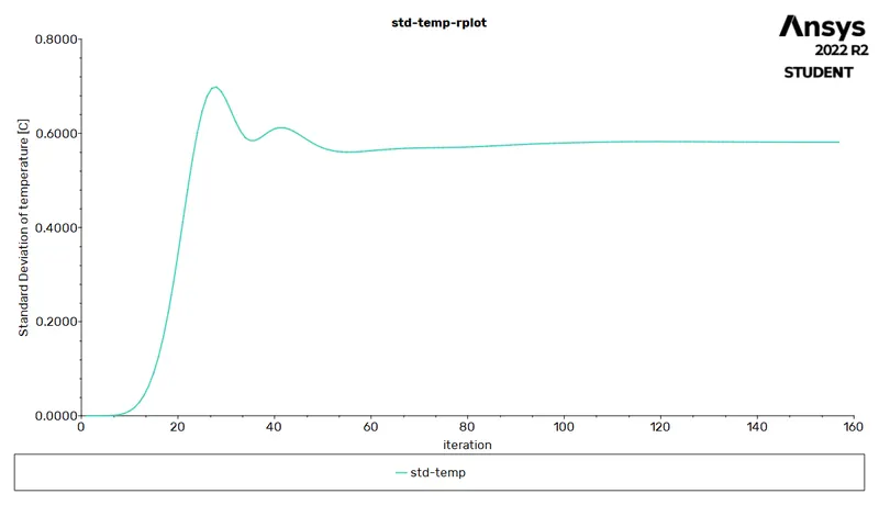
• Standard Deviation

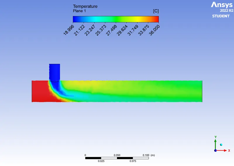
• Temperature contour

• Velocity contour

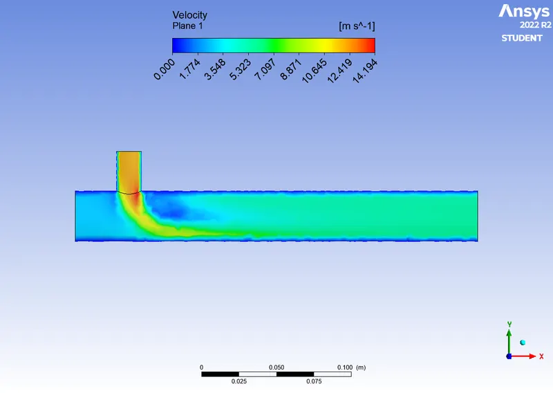
• Velocity Vector

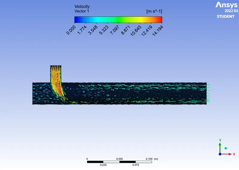
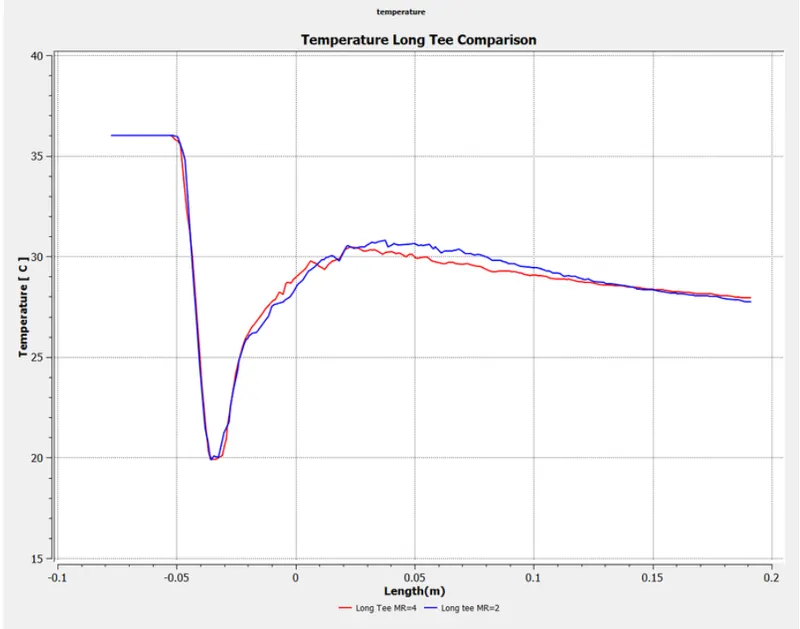
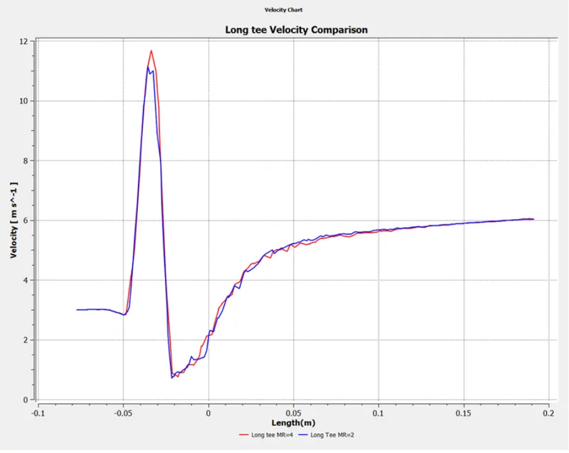
Comparison:

LONG TEE TEMPERATURE:

LONG TEE VELOCITY:

Anlytical Solution:

The temperature of the air at outlet can be given as,

Given Data:

Cases	Hot inlet velocity is 3 m/s and Cold inlet velocity is 6 m/s	Hot inlet velocity is 3 m/s and Cold inlet velocity is 12 m/s
Analytical Value TmixtureTmixture	Thot=36^oC Tcold=19^oC Ahot=901.3138mm^2 Acold=225.9823mm2 ρ=1.225kg/m3 Vcold=6m/s Vhot=3ms Tmixture=30.3^oC	Thot=36^oC Tcold=19^oC Ahot=901.3138mm^2 Acold=225.9823mm^2 ρ=1.225kg/m3 Vcold=6m/s Vhot=12m/s

Case	Average outlet temperature (c)	Number of iterations for convergence
Short tee- Momentum ration 2	30.26	192
Short tee- Momentum ration 4	27.61	160
Long tee- Momentum ration 2	20.23	200-210
Long tee- Momentum ration 4	20.23	200-210

CONCLUSION:

1. the length of the pipe increases the mixing has a lot of time and increases the temperature losing its main objective.

2. meshng has improved for both cases.

3.after comparing we can the increse the length dosednt have any effect on the mixxing of temprature at the outlet and increasing the velocity provides batter mixxing of temp at the outlet