Week 1- Mixing Tee

TITLE : - Mixing Tee 

Aim : - To perform the simulation on mixing tee and compare the mixing effectiveness for different conditions.

Problem Statement : - For this challenge, two versions of the mixing tee are created in which one of them is longer than the other. It is required to set up steady-state simulations to compare the mixing effectiveness when hot inlet temperature is 36⁰C & the Cold inlet is at 19⁰C. Use the k-epsilon and k-omega SST model for the first case and based on the judgment use the more suitable model for further cases and reasons for using it. 

1. Case 1 
   • Short mixing tee with a hot inlet velocity of 3m/s.
   • Momentum ratio of 2, 4. 
2. Case 2 
   • Long mixing tee with a hot inlet velocity of 3m/s.
   • Momentum ratio of 2, 4.

Momentum ratio = velocity at cold inlet / velocity at hot inlet

In a table, compare the following values from the 2 cases. 

1. Cell count
2. Average outlet temperature
3. Number of iterations for convergence

Expected results:

1. Velocity and temperature contour plots on the cut planes along and across the pipe.
2. Velocity and temperature line plots along and across the length of the pipe.
3. Perform Mesh independent study for any one case.
4. Discuss the effect of length and momentum ratio on results. 

For each simulation, you need to show the convergence plot.

Theory: -

1. Mixing tee is a pipe with T-Joint and the angle of the joint is 90 degrees. The mixing tee is used for applications of controlling the temperature at the user end in air conditioners , most of the application of mixing tee is in the nuclear power plant industries, power generation through steam, large scale research laboratories and mostly in cooling the system at required temperature. Other applications include in the heating and ventilating the system by mixing of two different fluids with same or different thermal and chemical properties. In the mixing tee, from the major end hot fluid flows and from the other end of joint at 90 degrees is inlet for cold fluid, thus this mixing of hot and cold fluids with different temperatures and velocities gives the required temperature of fluid at the outer end. This mixing also creates a turbulance inside the fluid volume of the mixing tee. 

2. The need of CFD simulation is to observe the effects of mixing of fluids inside the fluid volume in order to understand the flow behaviour during mixing, cyclic temperature fluctuations during mixing and to characterize the temperature variations inside the pipe wall itself. Turbulance will occur at the mixing region and the T- connections gets exposed to thermal fatigue which arises from low and high cycle tempertaure turbulances since there is major temperature difference between the fluids.

Procedure : - 

1. Open ANSYS Workbench. Import the Fluent model from the toolbox. Import the Geometry. Open SpaceClaim. It can be observed that in the spaceclaim the geometry imported is visible. Now to extract the fluid volume, go to toolbox at the top> Prepare> Volume Extract> Select the edges> Confirm the selection. This will extarct the fluid volume required. Now at the left top end shows the details. Hide the solid volume and use suppress for physics so that only the fluid volume is present for further operations. Close the Spaceclaim.

2. Open Meshing. The geometry from the spaceclaim will be imported into the ANSYS Meshing. Select the faces and give the named selection. There are two inlets and only one outlet and boundary as wall. Give mesh length (element size) and for quality use element quality. Then generate mesh. This will mesh the model into number of small elements. Moreover if inflation layer is to be given it can be done by defining the thickness of inflation layer and then generating the mesh.

3. After generating mesh update the mesh into the fluent software by right click and selecting update. Close the ANSYS mesh. Now open the ANSYS Fluent. The model will be loaded in the Fluent. Now Setting up domain> check mesh and see results in Console menu. If there are no errors or warnings then mesh is ok and can be proceed for solving.

4. Next step is setting up physics > Steady time,  Pressure based, Absolute velocity formulation, Models> energy equation on> Viscous> k-epsilon(2eqn) (realizable) / k- omega (2eqn) , Zones> Cell Zone> volume_volume> type>Fluid, Boundaries>

Inlet-x > velocity inlet> magnitude> 3 m/s> thermal> Temperature = 36^oC

Inlet- y> velocity inlet> magnitude> 12 m/s> thermal> Temperature = 19^oC

Outlet> Pressure outlet.

5. Solution> Reports > Definition> Area weighted average> Temperature > Surface outlet > Report file , Report plot, print to console on.

Same for area weighted average and standard deviation of temperature and velocity

Initialize > Hybrid initialization, then Calculate for 500 iterations. ANSYS fluent will solve for each iterations with defined boundaries.

This completes the solution (calculation) in fluent software. 

6. Start CFD Post in workbench in ongoing module. Create new plane and contour plots and the results can be observed.

This completes the procedure to perform simulation.

Calculations: -

Analytical calculations : -

Given Data: - 

1) Properties of air

Density of air = ρ_air = 1.225 kg/m³

Dynamic Viscosity of Air = µ_air = 1.7849 * 10 ^-5 kg/m*s

Specific heat of air = C_P = 1.006 kJ/kg K 

2) Mixing tee inlet and outlet end areas

Area at inlet- x = A_X = Area at outlet = A_O = 8.9979 * 10^-4 m²

Area at inlet- y = A_Y = 2.2484 * 10^-4 m²

3) Velocities

Velocity of hot fluid = 3m/s

Momentum ratio = Velocity at Cold inlet / Velocity at hot inlet

Given Momentum Ratio = 2

Then velocity of Cold fluid = 2*3= 6m/s

For momentum ratio = 4

Velocity of Cold Fluid = 12m/s

Now

Mass flow rate of hot fluid = Density* Area at inlet-x* Velocity of hot fluid

                                m _hot            = 1.225*8.9979 * 10^-4 * 3

                                m _hot            = 0.0040417 kg/s

Temperature of hot fluid = 36 + 273.15 = 309.15 K

A) For momentum ratio = 2

Mass flow rate of Cold fluid = Density * Area at inlet- y* Velocity of Cold Fluid

                                m _cold             = 1.225*2.2484 * 10^-4 * 6

                                m _cold             = 0.0020244 kg/s

Temperature of cold fluid = 19+273.15 =292.15 K

Using formula 

Substituting all values in above equation ;

T _mixture = 303.476 K = 30.3267 ^oC

B) For momentum ratio = 4

Mass flow rate of Cold fluid = Density * Area at inlet- y* Velocity of Cold Fluid

                                m _cold             = 1.225*2.2484 * 10^-4 * 12

                                m _cold             = 0.0040488 kg/s

Substituting all values in above equation ;

T _mixture = 300.64 K = 27.493 ^oC

Results : -

1. Mesh Independence study

Model: - k-epsilon realizable, Type of Tee: Short mixing Tee, Momentum ratio = 2

Sr. No	Element Size	Nodes	Elements	Outlet end temperature    (degree C)
1.	0.01	2812	12652	30.47
2.	0.005	3118	14100	30.39
3.	0.001	207683	635107	30.32

Smaller the element size, more finer the results.

 

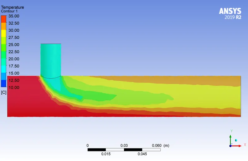
Figure 1: - Temperature contour with mesh element size = 0.01

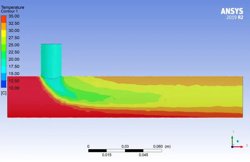
Figure 2: - Temperature Contour with mesh element size = 0.005

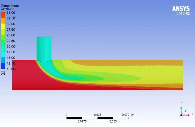
Figure 3: - Temperature Contour with mesh element size = 0.001

It can further be observed that there is smooth transition during mixing as element number is increased. This shows that more finer the mesh more are the accurate results.

Thus Mesh Element size was kept same for further cases = 0.001m

2. k-epsilon realizable v/s k-omega SST

k-epsilon realizable model is chosen for all simulations as compared to k-omega SST model as it can be seen that k-omega SST is used well for flow at near wall regions and k-epsilon realizable is for free suurface flow and far from wall region. In this as there is mixing of two fluids and flow is free surface flow k-epsilon works well as compared to k-omega. Figures 4, 5, 6, 7, 8 and 9 shows the comparision of results obtained from k-omega SST model and k-epsilon realizable model. It can be observed that since the reynolds number is much low thus k-epsilon model shows smooth results of temperature distribution and velocity contours. Moreover higher value of standard deviation of temperature is achieved for k-omega SST model as compared to k-epsilon realizable model which depicts that mixing is improper for k-omega SST model as compared to k-epsilon realizable model. 

Momentum ratio = 2

 

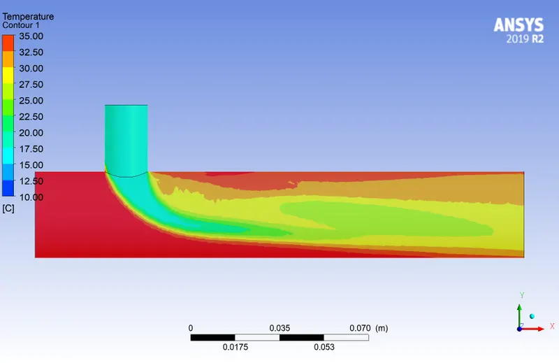
Figure 4a: - Temperature Contour with k-omega SST model 

Figure 4b: - Temperature Contour with k- epsilon realizable model

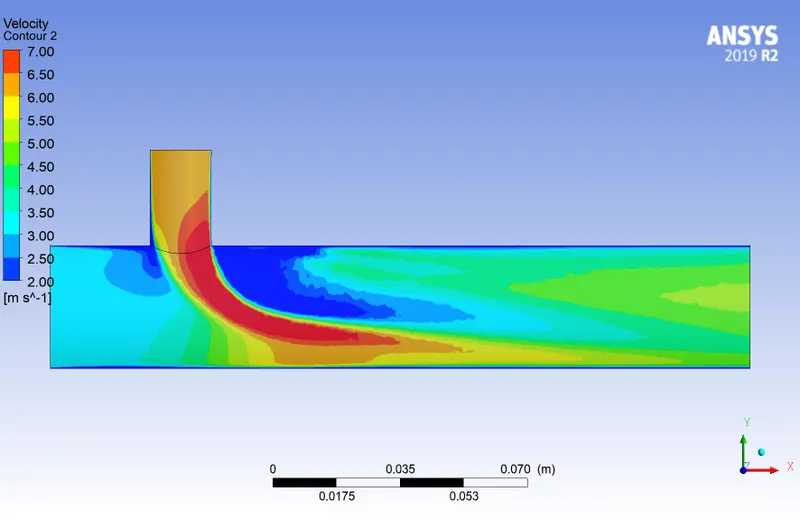
Figure 5a:- Velocity contour with k- omega SST model

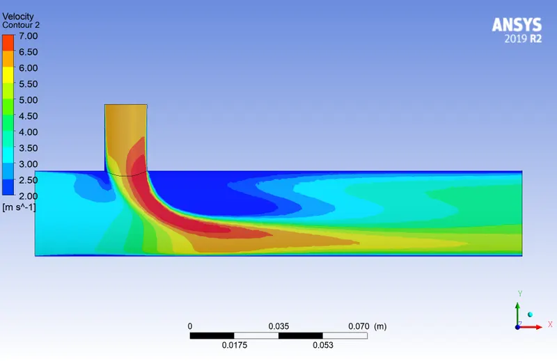
Figure 5b: - Velocity contour with k-epsilon realizable model

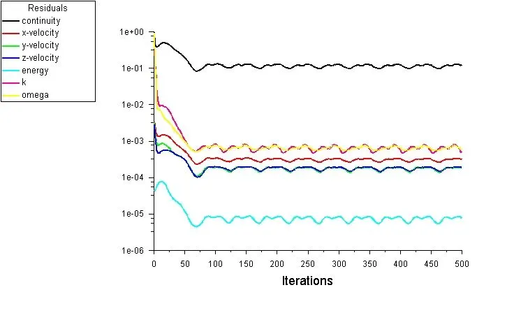
Figure 6a: -  Convergence plot for same number of iterations using k-omega SST model

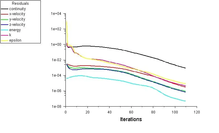
Figure 6b:- Convergence plot using k-epsilon realizable model

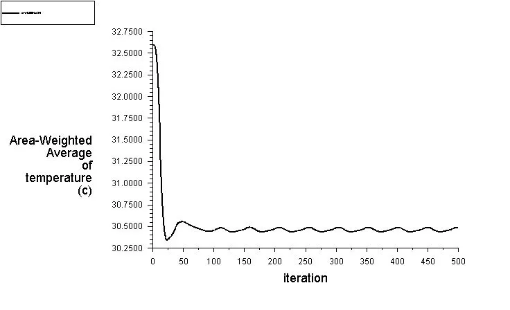
Figure 7a: - Area weighted average of temperature for k-omega SST model

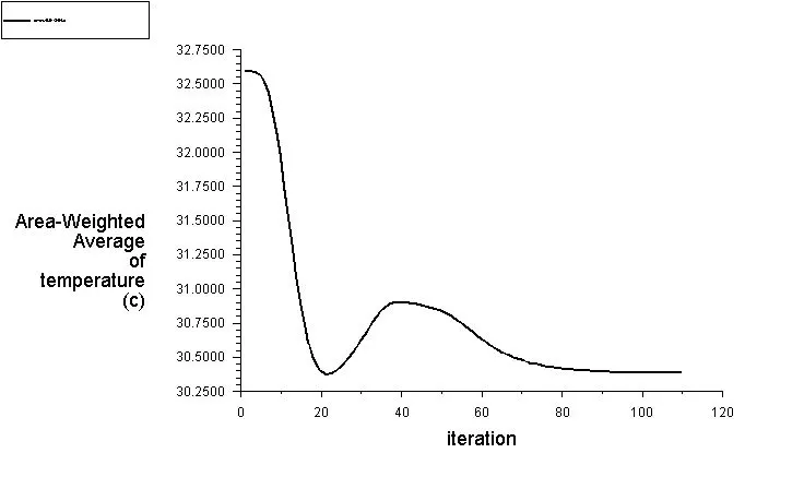
Figure 7b: - Area weighted average of temperature for k-epsilon realizable model

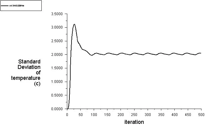
Figure 8a: - Standard deviation of temperature for k-omega SST model

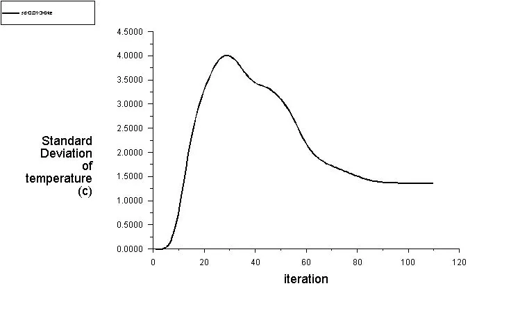
Figure 8b: - Standard deviation of temperature for k-epsilon realizable model

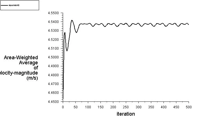
Figrue 9a: - Area weighted average of velocity for k-omega SST model

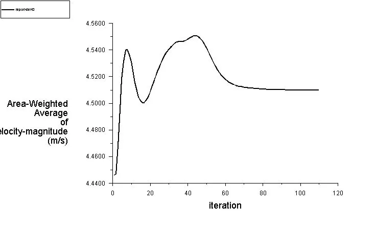
Figure 9b: - Area weighted average of velocity for k-epsilon realizable model 

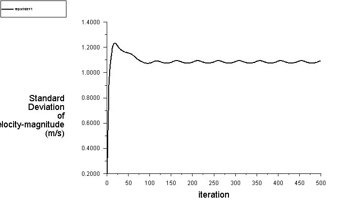
Figure 9c: - Standard deviation of velocity for k-omega SST model

 

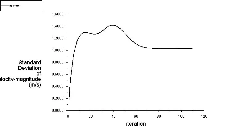
Figure 9d: -  Standard deviation of velocity for k-epsilon realizable model

3. Results for long mixing tee v/s short mixing tee

Momentum ratio= 4

It can be observed from figure 10, that there is no huge effect of length on the results. The results comes out to be  same.

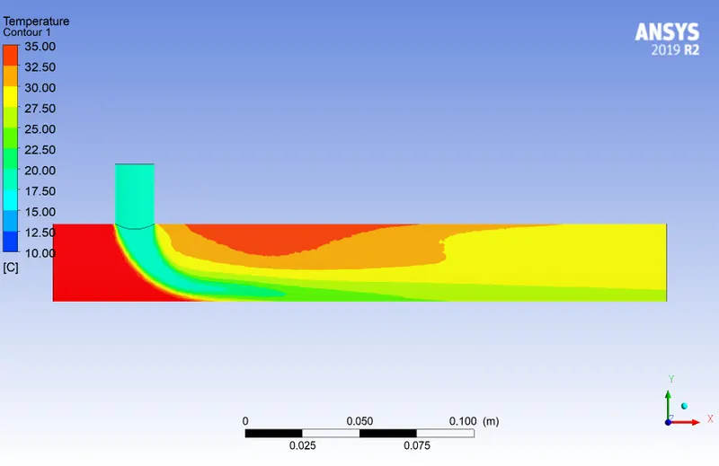
Figure 10a: - Temperature Contour of long mixing tee

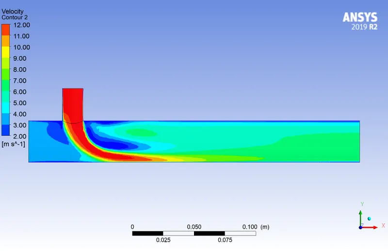
Figure 10b: - Velocity Contour of long mixing tee

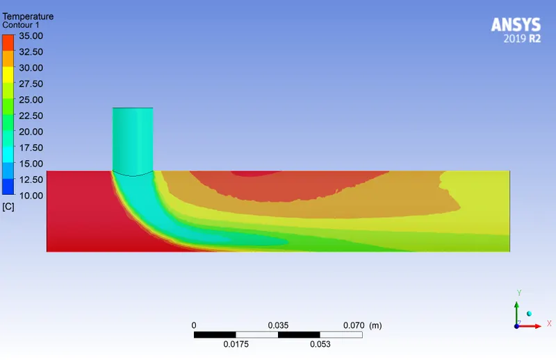
Figure 10c: - Temperature contour of short mixing tee

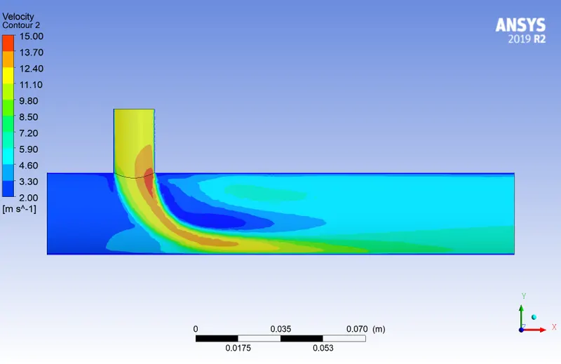
Figure 10d:- Velocity contour of short mixing tee

The temperatures obtained from the simulation for following momentum ratio: -

Momentum Ratio	Outlet temperature (deg C) (from simulations)	Type of mixing tee
2	30.38	Short
4	27.9	Short
2	30.4	Long
4	28.05	Long

Conclusion: -

The simulated and analytical results almost matches depicting that the simulation done is correct. k-epsilon model is chosen since the fluid mixing and flow is far away from the wall. There seems to be no huge variation in results if mixing tee used is long. Increase in velocity of cold fluid results in lowering of temperature. 

Learning outcomes: Use of ANSYS workbench, steps for simulation, effects of different models applied, understanding the results from contours.

Link to download the model

https://drive.google.com/file/d/1k8VCS6aNj6s7K2oGf-Pz4tzWc5lTpmbU/view?usp=share_link