Week 1- Mixing Tee

CFD SIMULATION OF MIXING TEE

AIM:

To perform steady state simulations and compare the mixing effectiveness with hot inlet and cold inlet temperature of 36℃ and 19℃ respectively for short tee and long tee with momentum ratios of 2 and 4 individually, given the inlet hot velocity is 3 m/s and compare the temperature, velocity contour plots and line plots.

INTRODUCTION:

• Discretization: The process of converting the partial differential equations into a system of algebraic equations is called discretization.
• Steady state simulations: The simulations where the flow characteristics do not change with time.
• Boundary conditions: These are the conditions that are specified to let know the solver that a particular location or a space has a particular value which is valid throughout the simulation.
• Initial conditions: These conditions are only specified to begin a simulation.

MIXING TEE:

Mixing Tee is a flow control device which consists of a ‘T’ joint used to mix two different fluids efficiently into a single stream. One of the most common applications is in air conditioner. Suppose the external temperature of air is around 35℃ and we need a lower temperature. By enforcing a stream of cool air at a higher velocity and mixing it with the stream of air at higher temperature using mixing tee, the temperature can be reduced considerably and by connecting this tee to the output of air conditioner we can expect the required temperature.

CASE 1: SHORT TEE:

1.a. MOMENTUM RATIO = 2

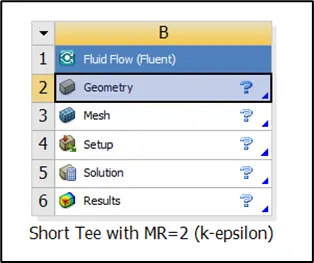
• Open ANSYS Workbench and drag ‘Fluid flow (Fluent)’ on to the interface.
• 
• Double click on ‘Geometry’ and ‘Space Claim’ will open. Import the geometry of mixing tee on to the interface.
• 
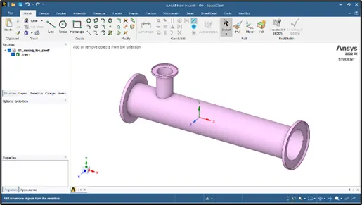
• Since the area of interest lies in evaluating the outlet temperature and the mixing efficiency (flow simulation), the solid geometry is not essential for the simulation.
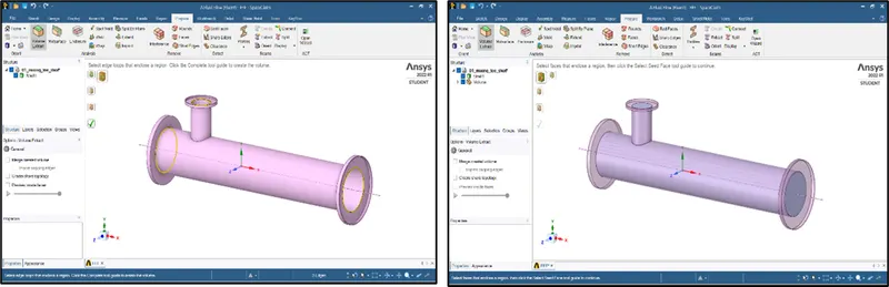
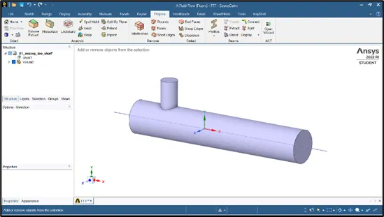
• Select ‘volume extract’ under ‘prepare’ menu, and with ‘select edges’ option enabled select the 3 circular edges and click on the 'green tick'.
• 
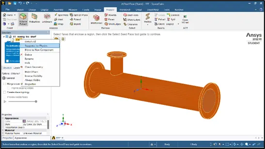
• Now uncheck the ‘shell’ option which hides the solid geometry. In order to avoid the presence of solid geometry for meshing, right click on ‘shell’ and select ‘supress for physics.’
• The volume has been extracted and is called wet volume and we can further proceed with meshing.
• 
• 
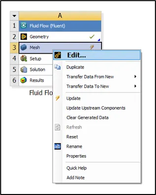
• Close the ‘Space Claim’ interface and open ‘ANSYS Mesher’ by right clicking on ‘meshing’ followed by ‘edit’.
• 
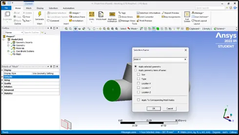
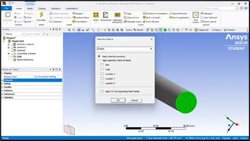
• Next step is to name the boundaries which is performed by enabling ‘face selection’ or using shortcut ‘CTRL+F’.
• The first inlet for hot air is selected and named as ‘Inlet-X’, by pressing ‘N’ which is a shortcut for ‘name selection’.
• 
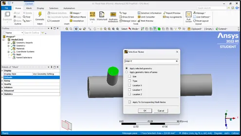
• The second inlet for cold air is selected and named as ‘Inlet-Y’.
• 
• The right-most face is selected and named as ‘Outlet’.
• 
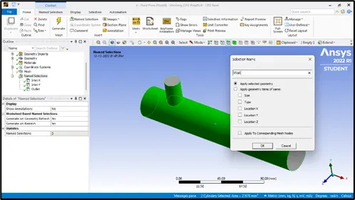
• Select both the cylinders and name them as ‘Wall.’
• 
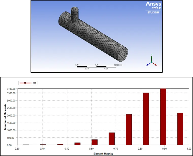
• The element size is taken as 10.219 mm (default), and the mesh is assigned by selecting ‘generate mesh’ option.
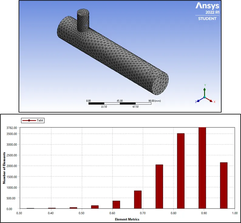
• The mesh metric is changed to ‘element quality’ to check the average element quality of the entire mesh.
• The element metrics histogram shows that the mesh is acceptable as it is greater than 5%.
• 
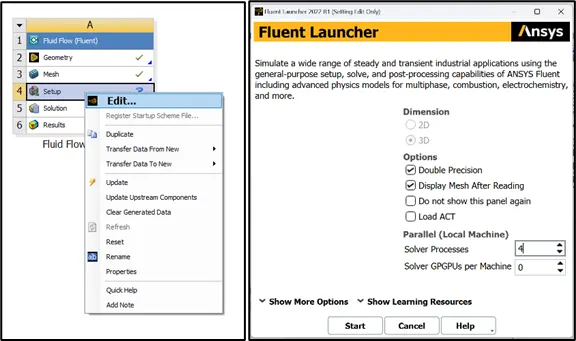
• Close ‘ANSYS Mesher’ and open ‘setup’ by right click and select ‘edit’ option.
• A window appears for launching ‘ANSYS Fluent’, check mark ‘double precision’ and set the ‘solver processors’ to 4, click ‘start’.
• 
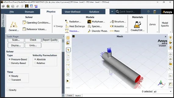
• Select ‘steady’, ‘absolute’ velocity formulation and ‘pressure-based’ under ‘solver’ and enable ‘energy’ under ‘models’ tab as we are interested to evaluate the outlet temperatures.
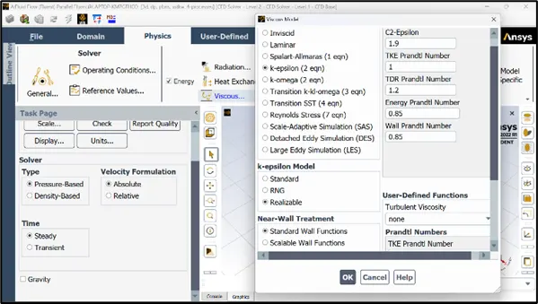
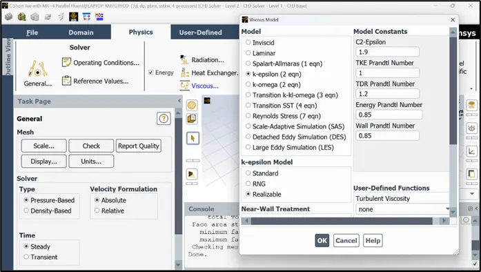
• Since the flow can be turbulent, select ‘viscous’ option under ‘models’ and select ‘k-epsilon’ realization model.
• 
• 
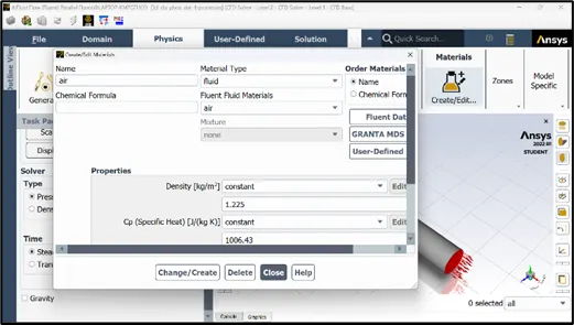
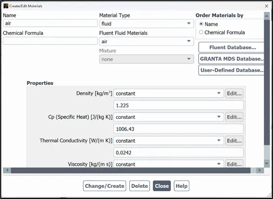
• Next set the material to ‘air’ by creating a new material under ‘create or edit material’.
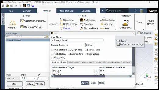
• To assign the boundary conditions, select ‘cell zones’ under ‘zones’ and click on edit by selecting the ‘volume’ option in the ‘task page’. Confirm with the material name as ‘air’ and type as ‘fluid’.
• 
• 
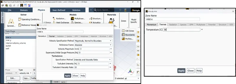
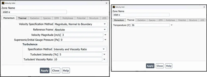
• Select ‘boundaries’ and click on ‘edit’ option by selecting ‘inlet-x’ and specify the velocity magnitude as 3 m/s. The temperature is set as 36℃ (309 K) in ‘thermal’ tab.
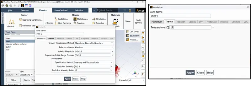
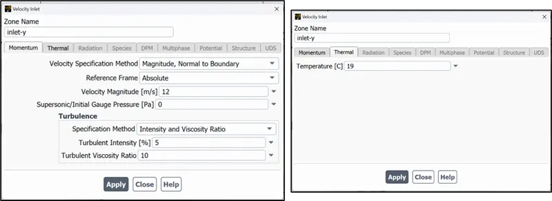
• Similarly, the values for ‘inlet-y’ are also specified. The velocity is calculated using the relation as follows,
• 
• 
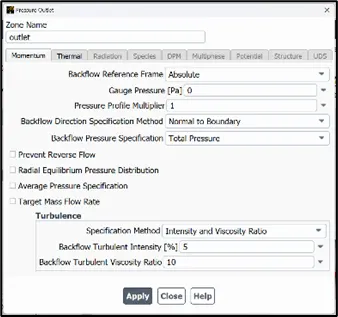
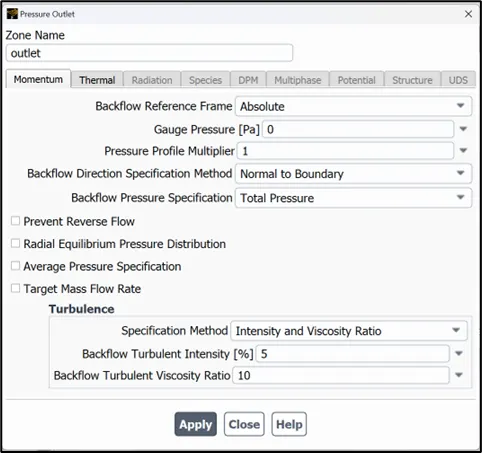
• The outlet conditions are set in default condition.
• 
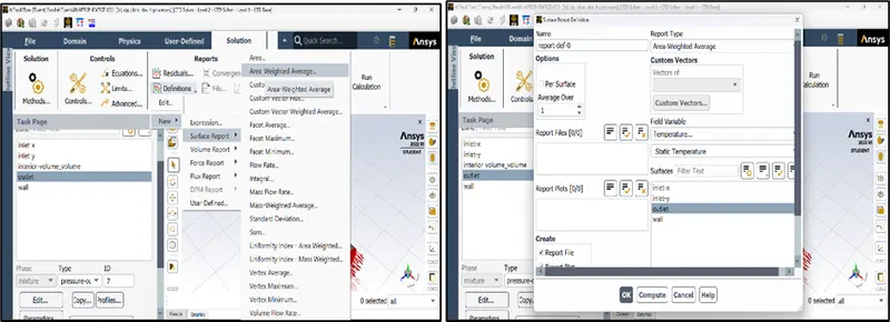
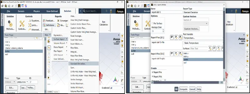
• Next go to ‘solution’ tab, and under ‘definitions’, select ‘new’ followed by ‘surface report’ followed by ‘area weighted average’.
• The area of interest is to evaluate the temperature at the outlet, select the ‘field variable’ as ‘temperature’ and face as ‘outlet’ as highlighted.
• Similarly, to view the ‘mixing efficiency’ select ‘standard deviation’ under ‘surface reports.’
• 
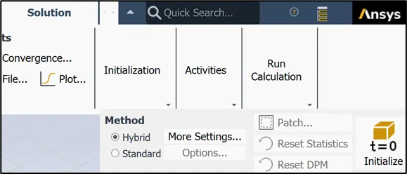
• The next step is to initialize the solution. The initialization is done using a ‘hybrid’ model to compute approximate values for velocity and pressure.
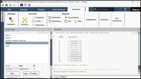
• Now click on ‘initialize’ and in console it can be seen that the initialization has taken place after 10 iterations because the hybrid initialization utilizes Euler’s method for 10 iterations.
• 
• 
• Enter the number of iterations as 300, and click ‘calculate’ to run the simulation.
• 
• 
• 
• 
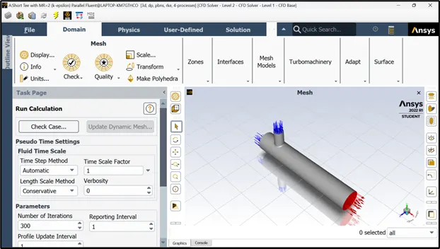
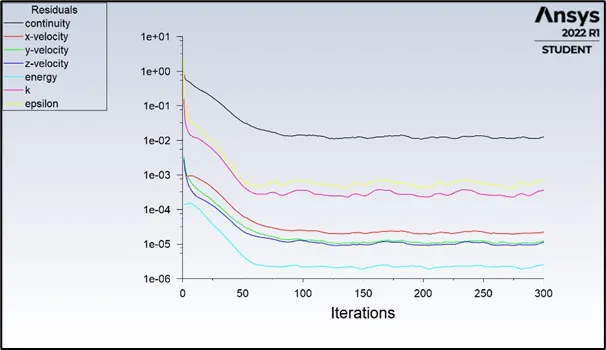
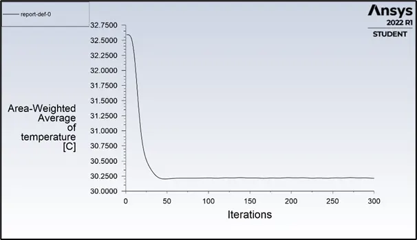
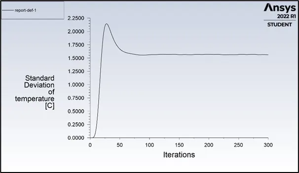
• Generally, the default setting in fluent for a solution to converge is when the residuals reach value of 1e^-3, which means that the simulation performed has generated the minimum statistics to generate an accurate result.
• The residuals have converged for all equations except for ‘continuity’. The temperature average weighted temperature at the outlet is 20℃ which has remained uniform from approx. 60^th iteration due to a lower value of standard deviation of 1.6℃.
• Close the ‘setup’ window and open the ‘results’ window by right click followed by a click on ‘edit’. This opens the post-processing window to view the results, plots of the simulation.
• 
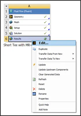
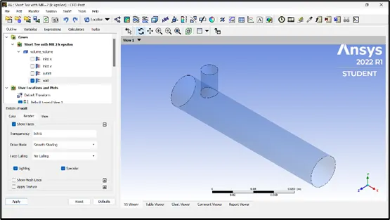
• Enable the ‘wall’ and double click. Under ‘render’ option, increase the transparency so that the contours are visible and click apply.
• 
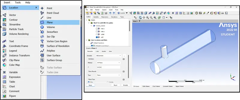
• To view the temperature and velocity variation throughout the length and across the wall, select ‘location’ under ‘insert’ menu and click on ‘plane.’
• Insert the plane in ‘XY’ plane with ‘Z=0’ and click on apply.
• 
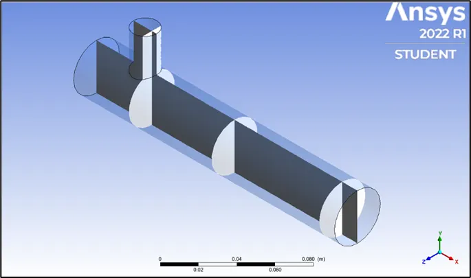
• To view the variation across the pipe, 4 different planes are considered in YZ plane at different locations as shown.
• 
• The temperature range to be viewed is changed to ‘user defined’ and set to 19℃ (min) and 36℃ (max). Under ‘text parameters’ of ‘appearances’ in ‘default legends view’, the precision is set to 2 and ‘scientific’ is changed to ‘fixed’.
• 
• 
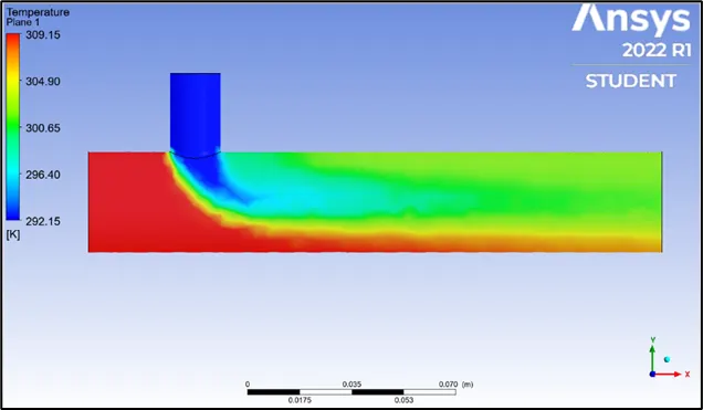
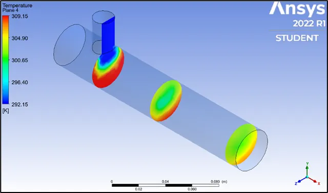
• It can be observed that at a momentum ratio of 2, the mixing of hot air and the cold air is not sufficient at the bottom to reduce the outlet temperature uniformly. The improper mixing is also due to insufficient heat exchange between fluids at sufficient velocity, which is evident from the plots as the temperature is still highest among majority of the locations (red contours).
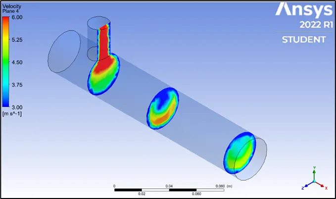
• Similarly, the velocity plots can be viewed changing the variable to velocity.
• 
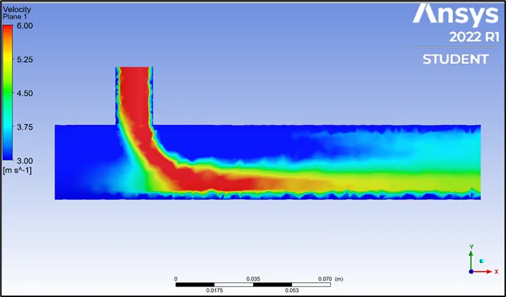
• The velocity of cold air is almost negligible or zero at the corners, upper and lower surface of the tee and after a certain distance have increased, which is due to no slip condition during flow of the fluid.
• 
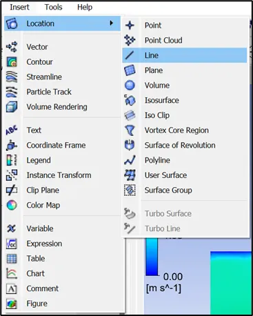
• To create line plot, insert ‘line’ option in ‘locations’ of ‘insert’ menu.
• Select the line type as ‘cut’ and click on apply.
• 
• 

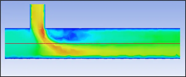
Temperature and velocity line plots

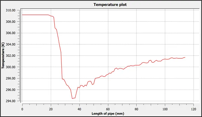
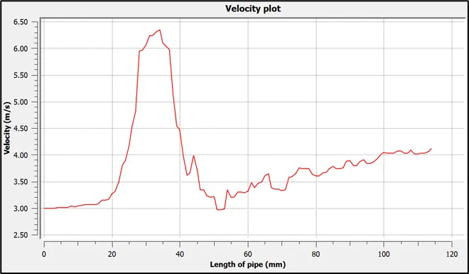
• The average temperature at the outlet is 25℃ and the velocity after mixing of both the fluids is 4.10 m/s.
• To compare the results of simulation with numerical method, we can use the following formula.
• 
• To calculate the mass flow rate of hot and cold air, click on ‘calculators’ and double click on ‘function calculators.’ Set the function as ‘mass Flow’ and location as ‘Inlet-X’ and click on calculate to obtain the mass flow rate of hot air as 00325806 Kg/s. Similarly, the mass flow rate of cold air is obtained as 0.00163376 Kg/s.
• 

Case 2: k – omega SST model:

• Drag and drop ‘Fluid flow (fluent) on to the interface. Click on ‘mesh’ of the earlier setup and drag it to connect with the ‘setup’ of the newly created analysis system. This ensures that the steps are transferred to the new system and the analysis can be directly begun by specifying the boundary conditions, analysis model to be considered etc.
• 
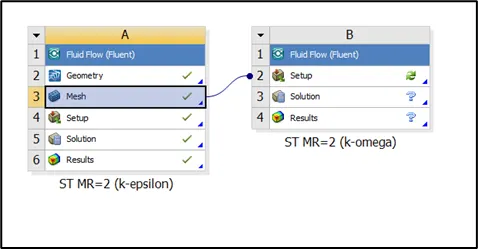
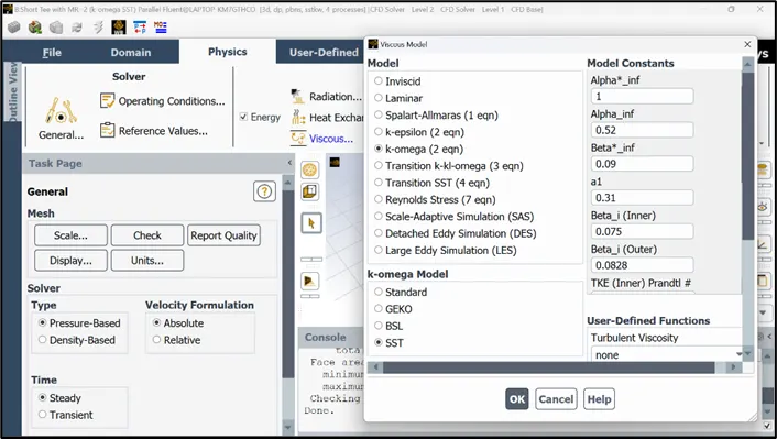
• Now right click on ‘setup’ and click on ‘edit’ to open the interface. Click on ‘mesh check’ in ‘setting up domain.’. In ‘setting up physics’ tab, enable the ‘energy’ (energy equations) and click on ‘viscous’ in models and select ‘k-omega SST’ model. Click OK.
• 
• Assign the material as ‘air’ and type as ‘fluid’ using ‘create/edit material’.
• Assign the boundary conditions, i.e., 3 m/s and 36℃ at inlet-X and 6 m/s and 19℃ at inlet-Y.
• Define the reports for ‘area weighted average temperature’ and ‘average standard temperature’ at the outlet.
• Initialize the solution using ‘hybrid’ method and set the number of iterations to 300 and click on calculate.

• Note: The images for the above steps are not included since they are a replica of the previous case.

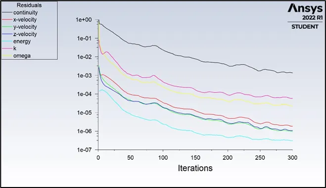
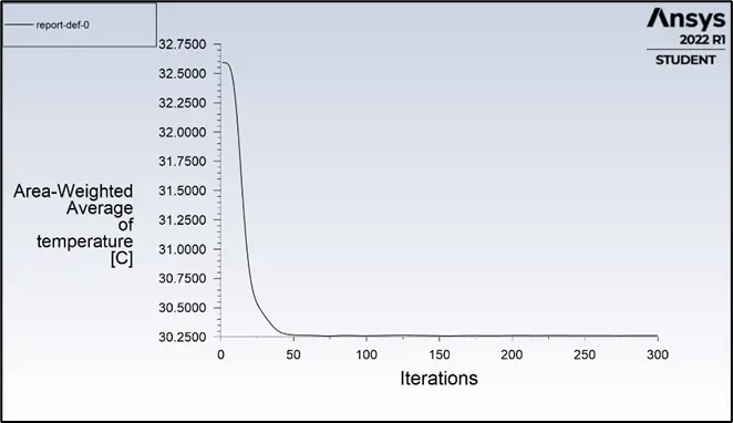
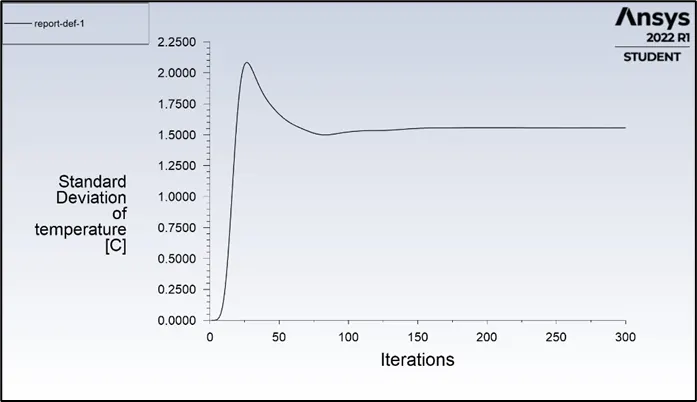
• The plots show that the solution is yet to converge even after 300 iterations. The average area weighted temperature at the outlet is 25℃ and the average standard deviation is 1.6℃.

Temperature contour plots:

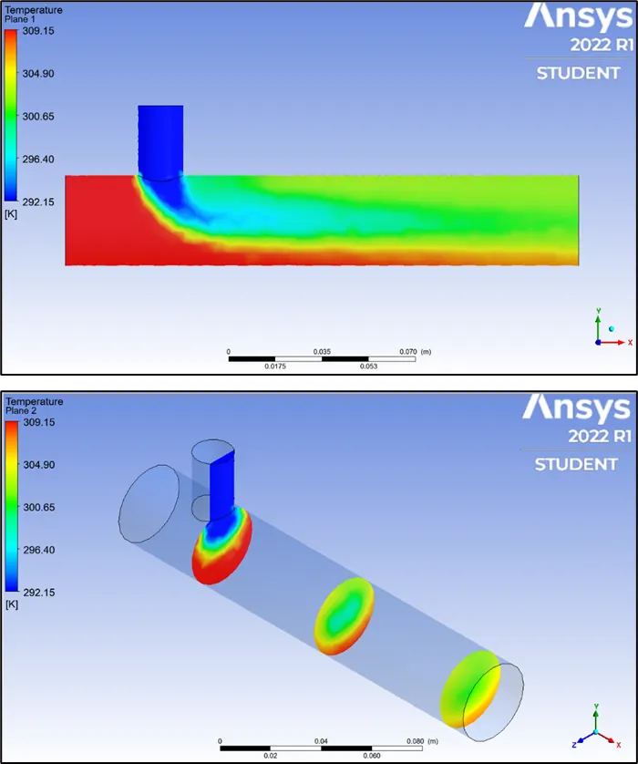
• The contour plots show that the temperature distribution at the outlet is not uniform, the temperature at the centre is approximately 27℃ and has increased away from the centre near to maximum value.

Velocity contour plots:

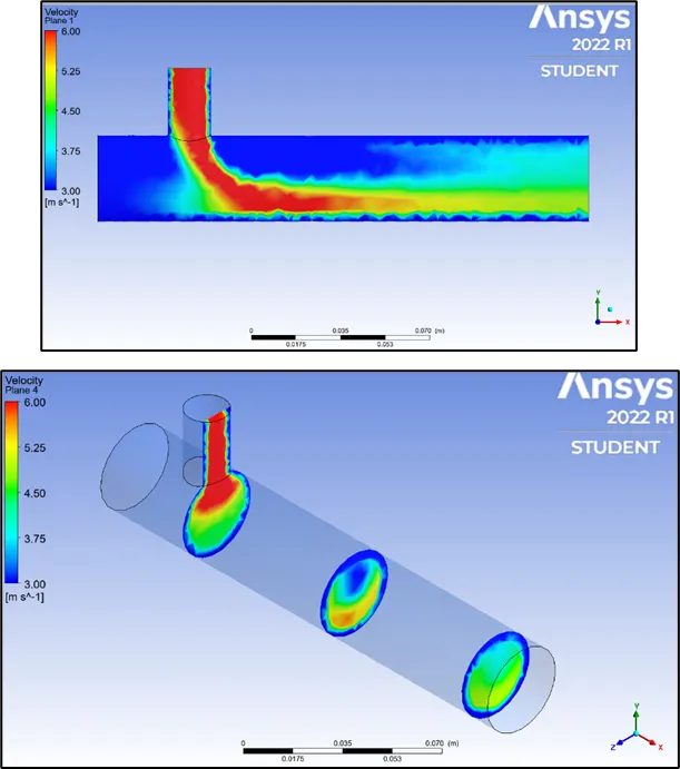
Temperature and velocity line plots:

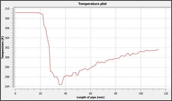
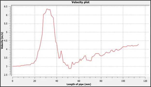
• The average outlet temperature after mixing is 25℃ and the maximum velocity after mixing is 4.3 m/s.
• The mass flow rate of hot air is 00325806 Kg/s and of cold air is 0.00163376 Kg/s. hence, the mixture temperature is 30.32℃.

Comparison between k-epsilon and k-omega SST model:

The comparison of plots show that the solution is nearly similar in both the cases but it gets converged more easily using ‘k-epsilon’ model whereas it is yet to converge in case of ‘k-omega SST’ model. Further, theoretically the ‘k-omega SST’ model is a combination of both ‘k-omega’ and ‘k-epsilon’ models which provides results for both conditions ‘near the wall’ and ‘away from the wall’ respectively, whereas the ‘k-epsilon’ model is often used in turbulent simulations away from the wall, which is the case here. Hence, based on these observations, for further simulations the ’k-epsilon’ model is used.

1.b. Momentum ratio = 4:

PRE-PROCESSING

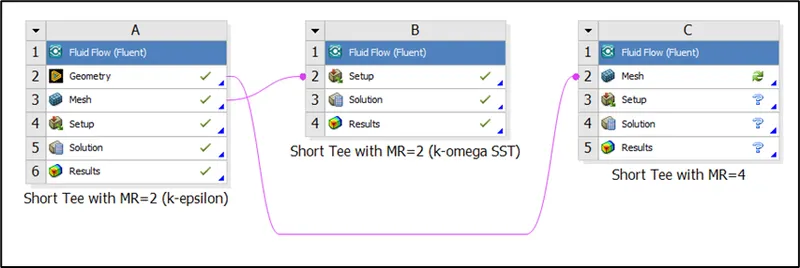
• Create a new project for ‘Fluid flow (fluent)’. Join the geometry setup of the previous case with the meshing setup of this case as shown.
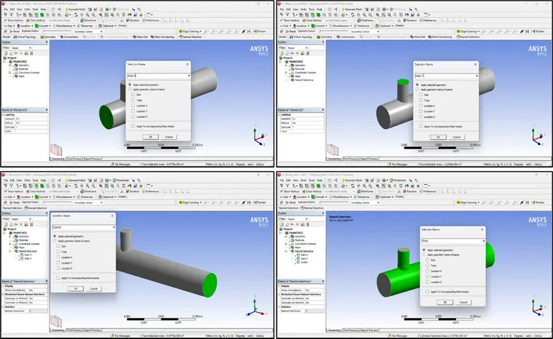
• Assign the boundary names ‘Inlet-X’, ‘Inlet-Y’, ‘Outlet’ and ‘wall’ using ‘named selection’ option with ‘face select’ feature enabled.
• 
• The mesh size is set as default (10.219 mm) and the ‘element quality’ is enabled under mesh metrics.
• 

SETTING UP PHYSICS FOR SIMULATION USING FLUENT SOLVER:

• Next step is to setup the geometry and provide the boundary conditions and initial conditions for the simulation.
• 
• Material assignment for the simulation
• 
• Initial conditions for the simulations

Inlet-X:

Inlet-Y:

Outlet:

• Creating reports for area weighted average temperature and average standard deviation to view temperature variation and asses mixing efficiency at the outlet.
• 
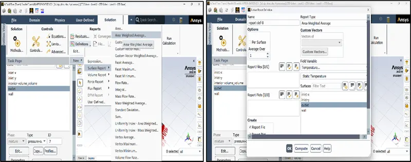
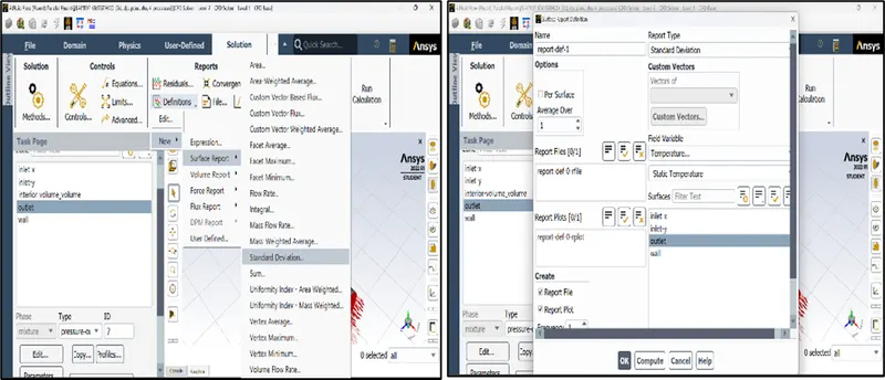
• The solution is initialized using hybrid initialization and further the simulation is run for 300 iterations to obtain the residual, average temperature and average standard deviation plot.
• 
• 
• 
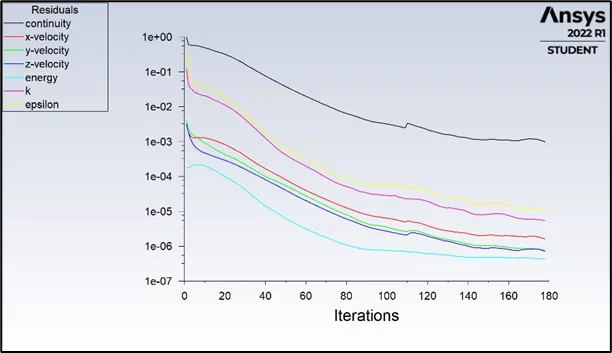
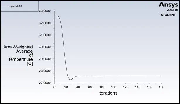
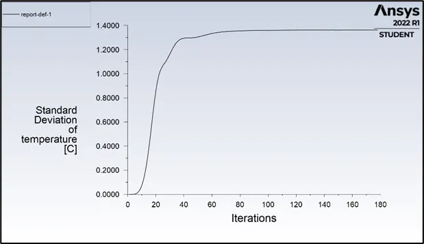
• The solution is converged after 178 iterations, and the area-weighted average of temperature is 27.5℃ which has remained uniform from approx. 60^th iteration for a lower value of standard deviation of 1.3℃.

POST PROCESSING

Temperature contour plots:

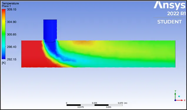
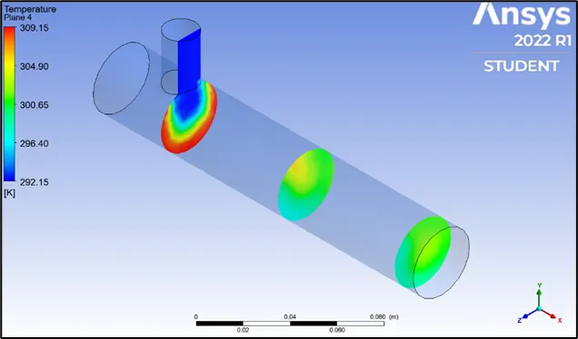
• In comparison with the case of momentum ratio = 2, the temperature is reduced significantly at the outlet due to the higher velocity of the cold fluid which helps in mixing the fluids more effectively along the length of the pipe.

Velocity contour plots:

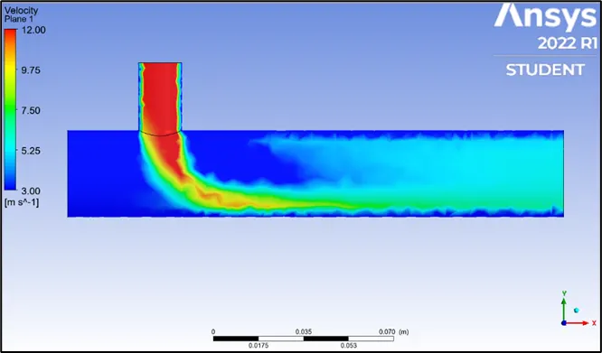
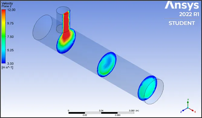
• The average velocity at the outlet has increased comparatively with the increase in momentum ratio which can be observed from the contours along and across the length of the pipe. The velocity near the walls is negligible and as we move away from the wall, the velocity gradually increases due to no-slip condition.
• 

Temperature and velocity line plots:

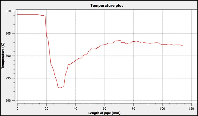
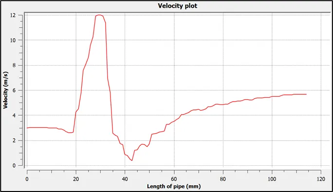
• The average temperature at the outlet is 5℃ and the velocity after mixing is 5.5 m/s.
• Theoretically,

m_cold = 0.00325806 Kg/s

m_hot = 0.00326751 Kg/s

CASE 2: LONG TEE

2.a. Momentum ratio = 2:

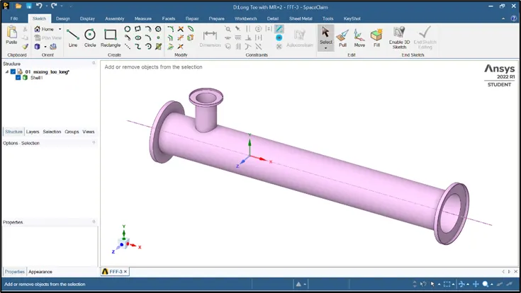
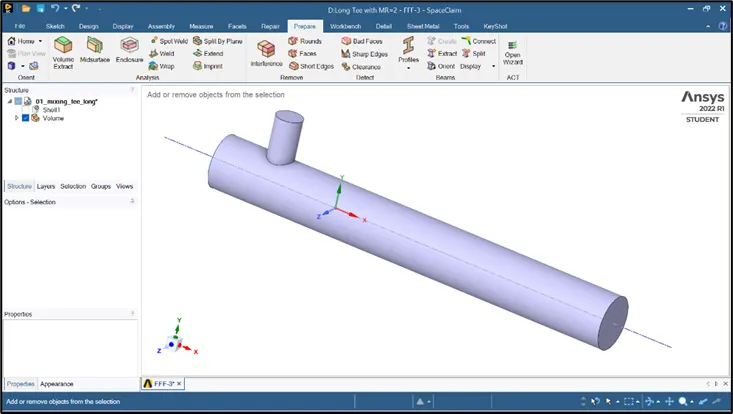
• Import the long tee model and extract the wet volume for the CFD analysis.
• 
• 

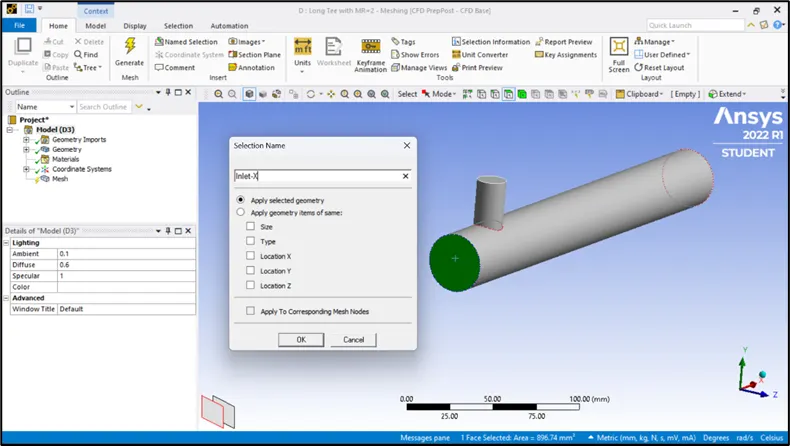
Assign the boundaries and meshing the component

Inlet-x:

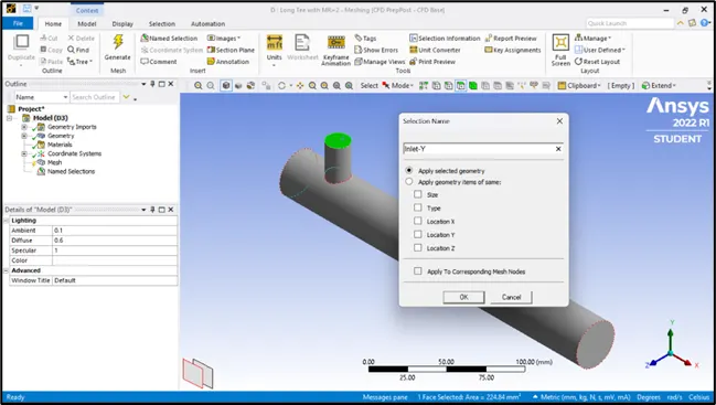
Inlet-Y:

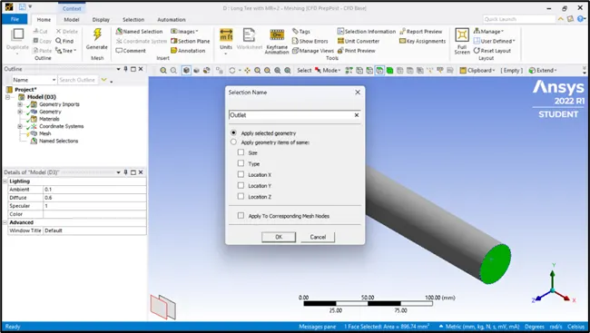
Outlet:

Wall:

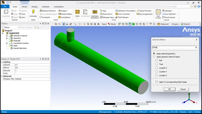
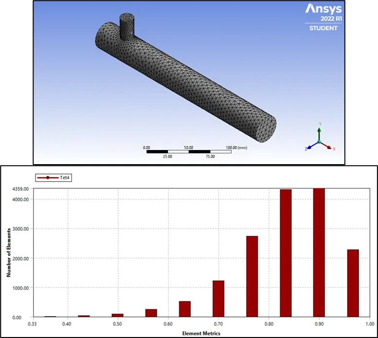
• The mesh is assigned with a default element size of 10.219 mm by enabling the element quality under the mesh metric.
• 
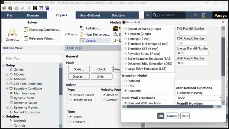
• Right click on ‘setup’ and click on ‘edit’ to open the interface. Click on ‘mesh check’ in ‘setting up domain.’. In ‘setting up physics’ tab, enable the ‘energy’ (energy equations) and click on ‘viscous’ in models and select ‘k-epsilon realizable’ model. Click OK.
• 
• Assign the material as ‘air’ and type as ‘fluid’ using ‘create/edit material’.
• Assign the boundary conditions, i.e., 3 m/s and 36℃ at inlet-X and 6 m/s and 19℃ at inlet-Y.
• Define the reports for ‘area weighted average temperature’ and ‘average standard temperature’ at the outlet.
• Initialize the solution using ‘hybrid’ method and set the number of iterations to 300 and click on calculate.
• 
• 
• 
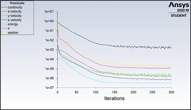
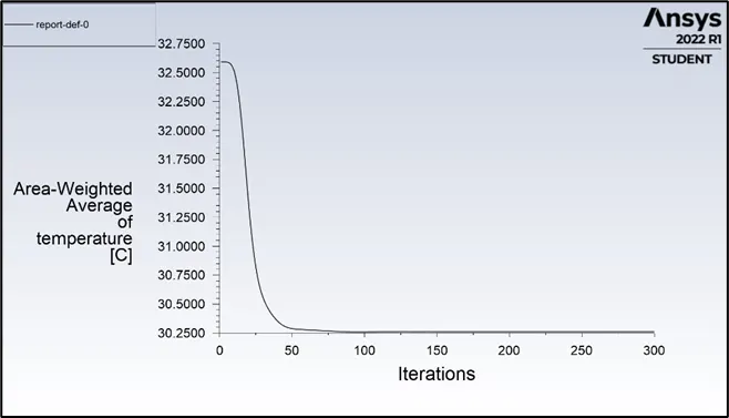
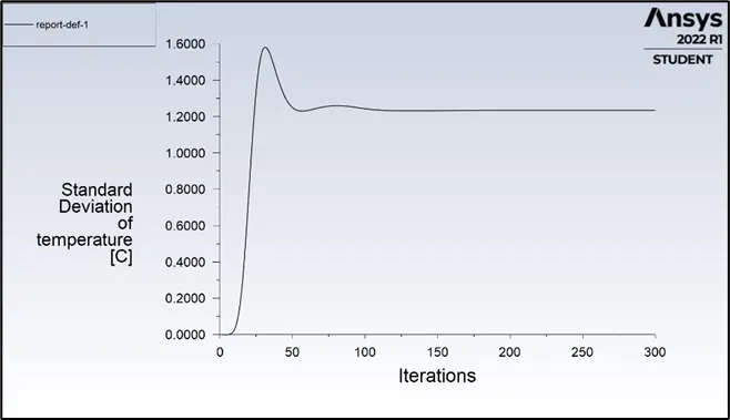
• The residuals have converged at approx. 200 iterations except for ‘continuity’. The area weighted average of temperature at the outlet is 25℃ with a lower standard deviation of 1.25℃.

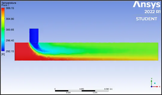
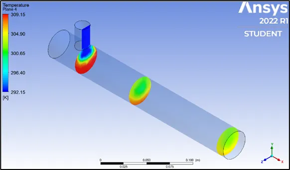
Temperature contour plots:

Velocity contour plots:

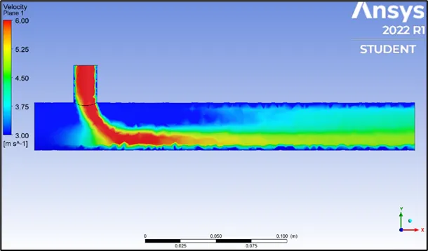
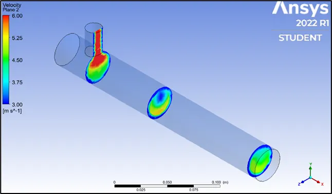
Temperature and velocity line plots:

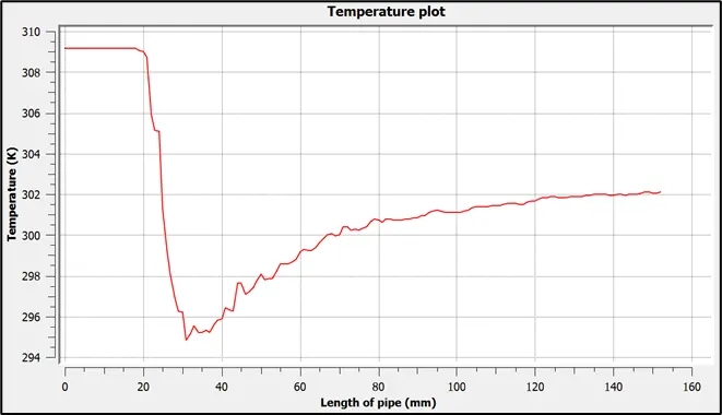
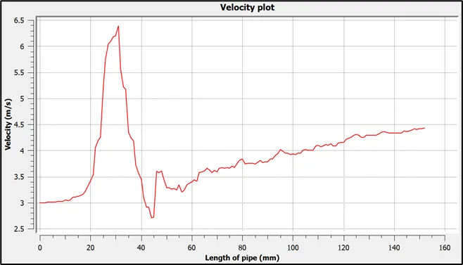
• The average temperature at the outlet is 25 ℃ (309 K) and the velocity of the mixed fluid is 4.4 m/s.

Theoretically,

m_cold = 0.00325805 Kg/s

m_hot = 0.00163375 Kg/s

2.b. MOMENTUM RATIO = 4

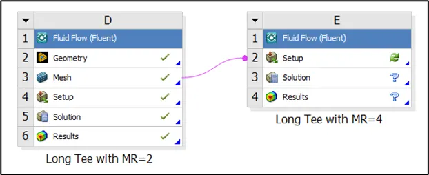
• Create a new project ‘Fluid flow (fluent)’ and connect the ‘mesh’ of the previous case with the ‘setup’ of the new project since the steps till volume extraction and meshing remain the same.

• The simulation can now be directly begun with the ‘setup’.
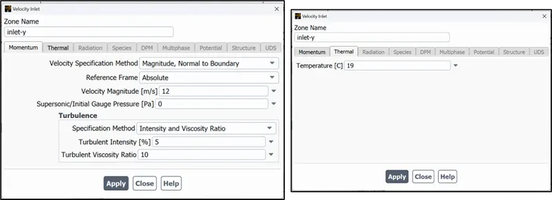
• Each of the steps are identical as that of in the previous case except for change in momentum ratio, which changes the value of the ‘inlet-y’ velocity as shown.

• The reports are defined for ‘area weighted average temperature’ and ‘standard deviation’ to evaluate the average temperature at the outlet and mixing efficiency.
• The initialization of solution is done and is run for 300 iterations.
• 
• 
• 
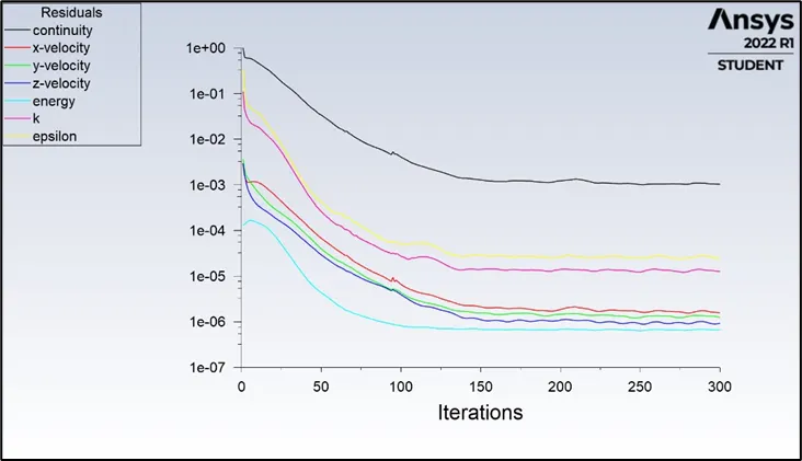
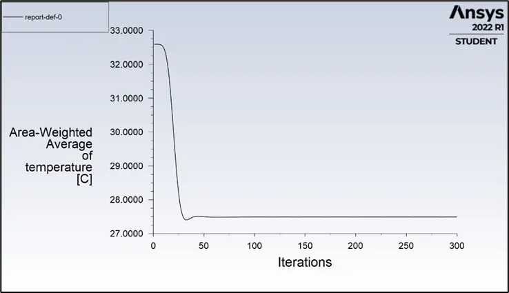
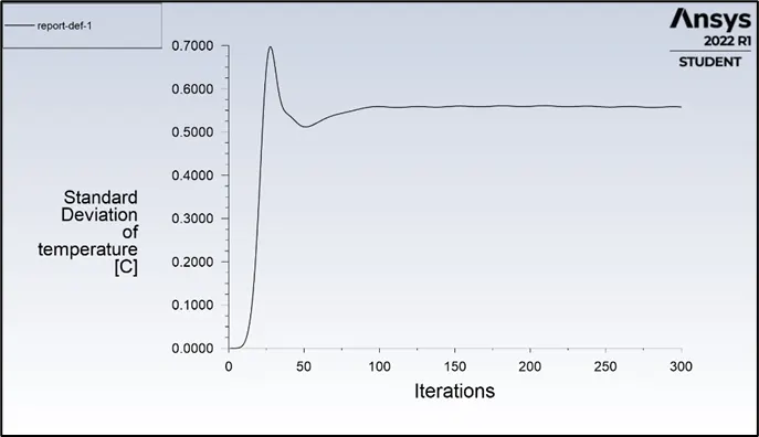
• The residuals have converged approx. at 200 iterations except for ‘continuity’. The area weighted average temperature at the outlet after mixing is 27.45℃ and is uniform from 60^th iterations which is due to a very low value of standard deviation of 0.55℃ which shows that the mixing of fluids is significant.

Temperature contour plots:

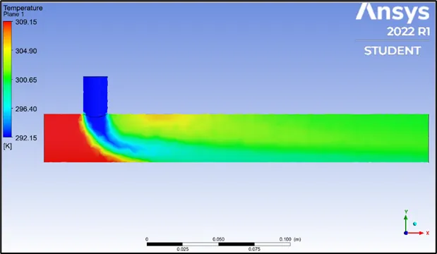
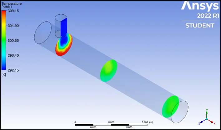
The contours show that the temperature has been reduced greatly at the outlet which is due to the higher velocity of cold fluid ensuring proper mixing along and across the length of the pipe.

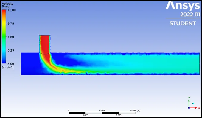
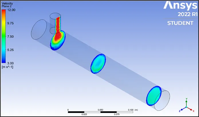
The velocity is observed to be increasing along the length of the pipe for a certain distance and gradually become stable further which is due to no slip condition. The plots across the length of the pipe also show that the velocity is higher at the centre and least near the walls of the pipe.

Temperature and velocity line plots:

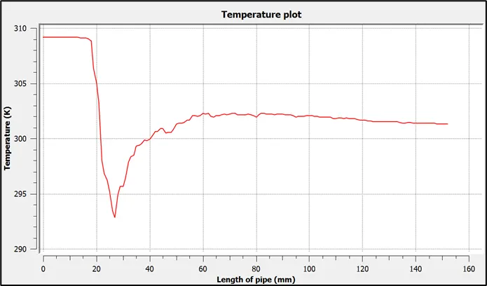
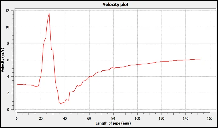
• The average temperature at the outlet of the mixed fluid is 45℃ and the velocity of the mixed fluid is 6.1 m/s.

Theoretically,

m_cold = 0.00325806 Kg/s

m_hot = 0.00326751 Kg/s

MESH INDEPENDENT STUDY:

• The mesh independent study is done to compare the results for different mesh element sizes. Since accuracy of the solution for FEA depends on the discretization of the domain, it is necessary that a proper mesh size is selected. Finer will be the mesh more will be the accuracy of the solution but the computational time will be more and vice-versa. Hence to overcome this, we perform mesh independent study to determine the appropriate mesh size to be selected for the mesh without compromising for the accuracy and reducing the computational time.
• The following study is performed for long tee with momentum ratio of 4 and the mesh element sizes are selected as 10.219 mm (default), 5 mm and 2 mm.

Mesh element size (mm)	Nodes	Elements	CFD solution of average temperature at outlet (℃)	Theoretical average temperature (℃)	Average standard deviation (℃)	No. of iterations to converge
10.219 (default)	3499	15727	27.45	27.48	0.55	178
5	4012	18100	27.50	27.49	0.50	328
2	28450	140990	27.50	27.52	0.7	233

• From the above table we can observe that more accurate results are obtained as the mesh becomes finer. The only compromise that has to be made is that finer will be the mesh higher will be the computational time due to increased number of elements. Hence, proper mesh element size must be used as per the demand of the application.

COMPARISON BETWEEN PERFORMANCE OF SHORT TEE AND LONG TEE:

Model	Momentum ratio	Nodes	Elements	Average outlet temperature (℃)		Average outlet velocity	Standard deviation (℃)	No. of iterations to converge
				CFD solution	Calculated value
Short Tee	2	2840	12780	30.20	30.32	4.30	1.60	≈200
	4	2840	12780	27.50	27.48	5.5	1.30	178
Long Tee	2	3499	15727	30.25	30.32	4.4	1.25	≈200
	4	3499	15727	27.45	27.48	6.1	0.55	≈200

The results show that there is no such difference in the capacity of the tees to reduce the outlet temperature, rather the velocity of the cold fluid has a vital role in proper mixing of fluids in order to obtain the required temperature. Also, in case of long tee, better mixing is observed as indicated by lowest standard deviation which can be due to the additional mixing occurring due to diffusion.

EFFECT OF LENGTH AND MOMENTUM RATIO:

From the results obtained, the length of the tee is not influential in reducing the output temperature of the mixed fluid since both the tees at similar momentum ratios have nearly identical results. Further, the long tee can be considered as a better option since it allows better mixing due to diffusion as indicated by least standard deviation value (also evident from the mesh independent study).

The momentum ratio is crucial factor for proper mixing of fluids as it can be observed that by increasing the momentum ratio by a multiple of 2, there is a significant decrease in output temperature approx. by 2.7℃ in both the cases.

CONCLUSIONS:

• The results shows that the ‘k-epsilon realization’ model is effective for predicting the behaviour of temperature throughout the mixing tee.
• The contour plots and line plots of all the cases are more or less the same for a given momentum ratio, which clearly indicate that the momentum ratio is a crucial factor for mixing of two fluids effectively.
• The mesh independent study shows that finer the mesh element size, longer will be the computational time but will provide more accurate results.

https://drive.google.com/file/d/181tBldEyLuDkIjQbfJuDWXjJvZ6Rthyp/view?usp=share_link