Week 1- Mixing Tee

Objective: To set up steady state simulations to compare the mixing effectiveness for given inlet and outlet temperatures. And to compare it for short and long pipes.

CASE 1:

• Short mixing tee with a hot inlet velocity of 3 m/s
• Momentum ratio 2,4

CASE 2:

• Long mixing tee with a hot inlet velocity of 3 m/s
• Momentum ratio 2,4

SImulation :

1. M.R=2 short pipe
2. M.R=4 short pipe
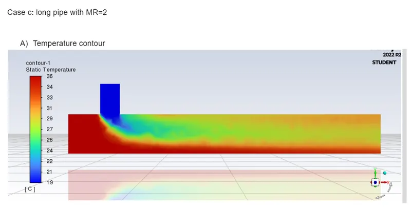
3. M.R=2 long pipe
4. M.R=4 long pipe

There are two models to get the solution to converge. The k-epsilon and k-omega are considered for the given problem. Both the methods have their own pros and cons. The K-epsilon model predicts the behavior of flow very well far away from boundaries and k-omega captures it near the wall.

Now in this case we will use both the methods for the same simulation. Hence we will take simulation a) for our study.

Here both the k-epsilon and k-w model will be taken into consideration for convergence study.

General Procedure:

1. Open the ansys workbench and select mesh from the component system. Drag and drop it in the workspace.
2. Right click on the geometry and select import.Import the step file from your location and open it in spaceclaim.
3. Prepare the geometry by extracting the edges from the cad.Suppress the actual model.Close spaceclaim
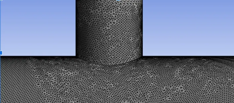
4. Open the meshing software. Click on generate mesh ,you will get default meshing.Now change the element size to 0.5mm and update the mesh.To check the meshing inside the geometry take a section plane along the length of the pipe.
5. Create the name selection by selecting the faces such as inlet-x,inlet-y,outlet and wall.This names will be helpful while providing the boundary conditions.
6. Now select Fluent from the analysis system and drag-drop it. Attach the mesh to this Fluent box so that this same mesh can be used for k-epsilon and k-w models.
7. Open Ansys Fluent by selecting setup.
8. Select the physics tab. In that select the viscous model and then select the k-epsilon turbulence model.Tick the energy box so that the energy equation gets activated to find out the temperature.
9. Select the material as air and close the tab.Click on boundary conditions and provide the boundary conditions at inlet. Select cell zones and make sure that volume is fluid or else simulation will not start.
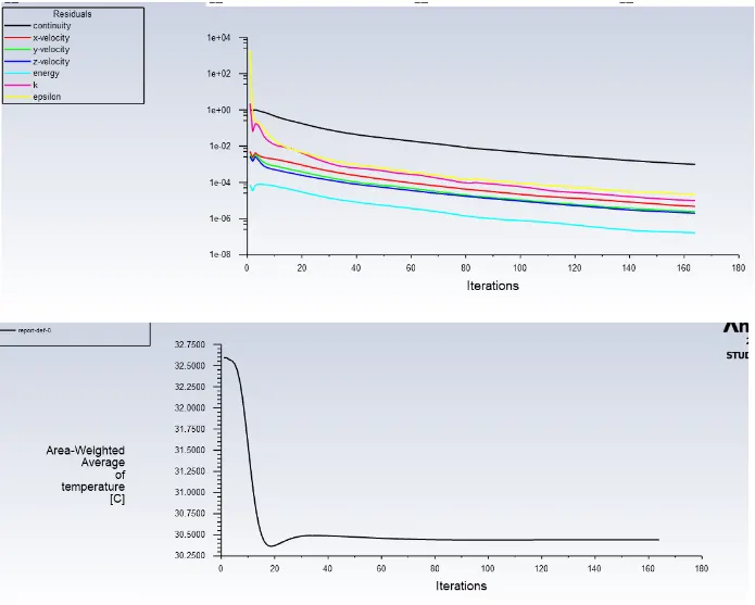
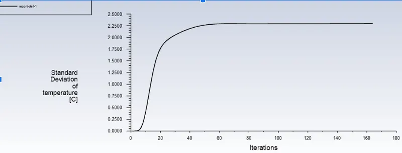
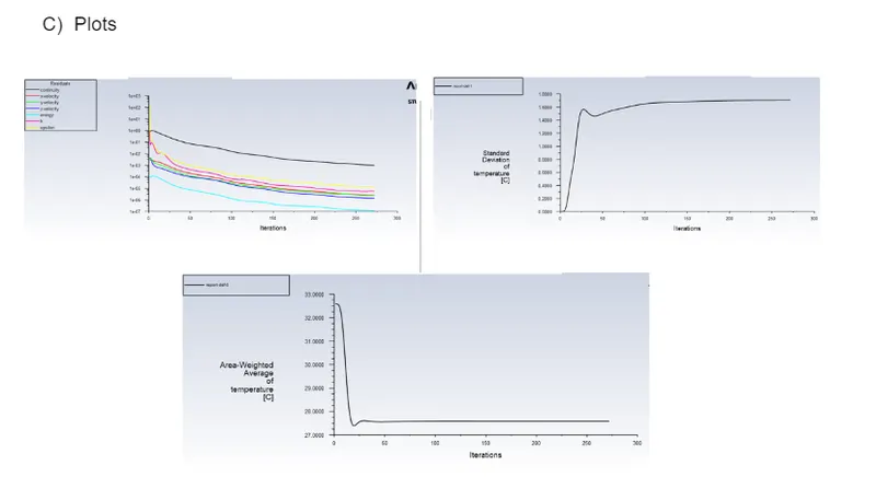
10. Go to the solution tab and select methods. Click on higher order relaxation so that solution can converge. Select hybrid initialization, and click on initialize.Now provide number of iterations. Before starting the calculation click on definition and select area weighted average and standard deviation report for temperature.
11. After calculation is completed,close the fluent and open cfd post.
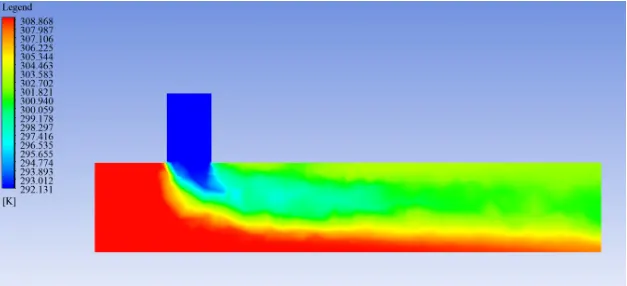
12. Here add one plane along the length of pipe so that temperature and velocity contours can be plotted.

Repeat the above process for other cases.

Below are the images of various steps followed.

A)Meshing

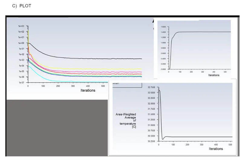
B)Plots

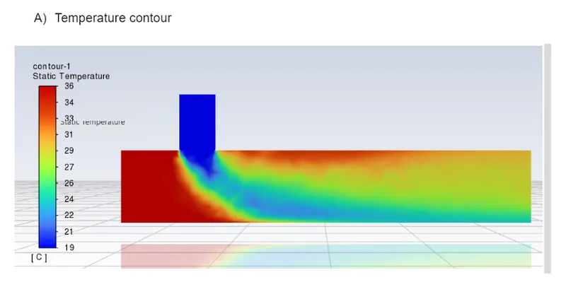
C) Temperature contour

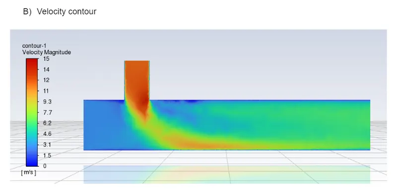
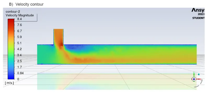
D) Velocity contour

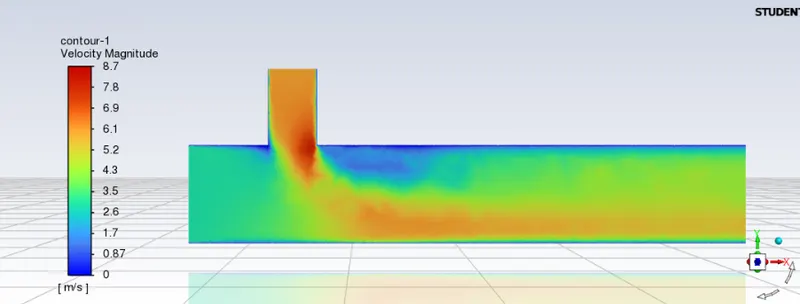
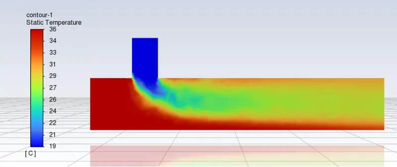
Similarly for k-omega model:

A) Temperature contour

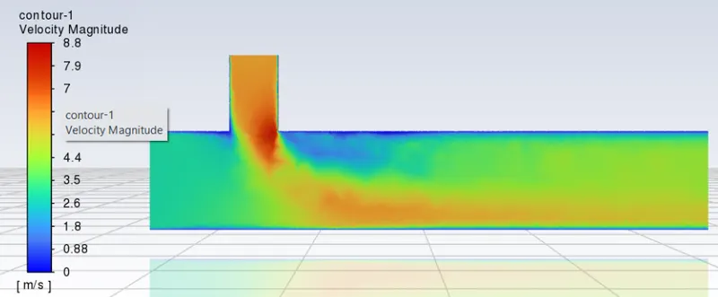
B) Velocity contour

C) PLOTS

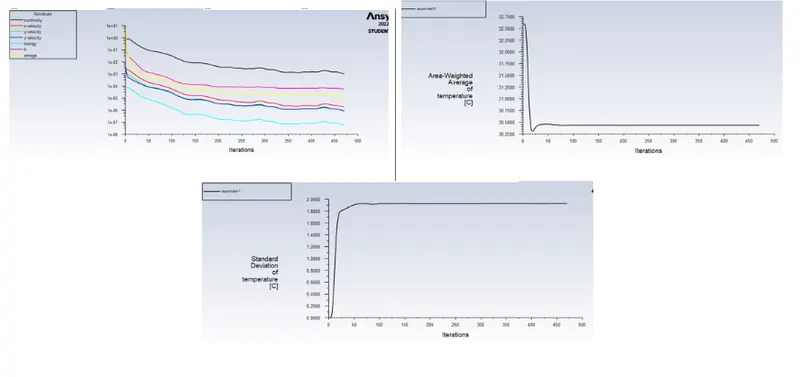
As pointed out earlier k-epsilon model is more suitable for capturing the flow behavior away from boundary and k-omega is suitable for capturing the flow behavior near the boundary.So in this case we want to see the flow behavior away from the boundary.Therefore k-epsilon model is used for further simulations. You can observe that the no.of iterations required to converge the solution is less in k-epsilon than in k-omega.

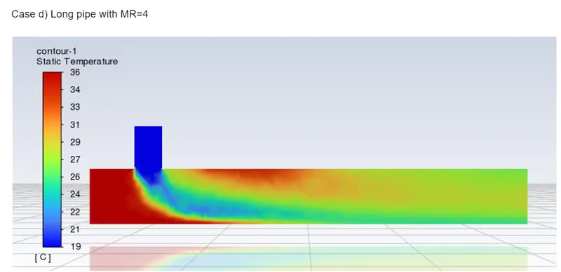
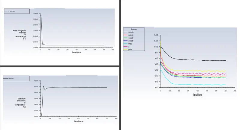
Next we will use the MR=4 model for the simulation purpose alongwith k-epsilon model;i.e case b).

Below is the table denoting the various aspects of each simulation

SHORT PIPE					Actual temperature
MODEL	k-epsilon model		k-omega model
MR=2	T= 30.24°C	CONEVERGED AT 164th iteration	T= 30.261°C	CONEVERGED AT 470th iteration	29.88 °C
	no. of iterations=300		no. of iterations= 600
	no. of cells= 497486		no. of cells= 497486
MR=4	T= 27.56°C			CONEVERGED AT 272nd iteration	27°C
	no. of iterations=300
	no. of cells= 497486
LONG PIPE					Actual temperature
	k-epsilon model
MR=2	T= 30.4°C			CONEVERGED AT 350th iteration	29.88 °C
	no. of iterations=400
	no. of cells= 163556
MR=4	T= 27.55°C			CONEVERGED AT 505th iteration	27°C
	no. of iterations=500
	no. of cells= 163556

Conclusion

1. k-epsilon model is the most suitable model.As it predicts the flow behaviour much accurately and precisely which is away from the wall.Also the number of iterations required to converge are less in k-epsilon model.

2.The length of pipe is independent of the mixing,therefore as seen from the temperature and velocity contours one can see that for proper mixing short pipe with momentum ratio of 4 is more suitable.

3. Also the time required for convergence or number of iterations are much greater than short pipe even though the number of cells are less as compared to above case.