Week 1- Mixing Tee
Mixing Tee Simulation
AIM: To set up steady-state simulations to compare the mixing effectiveness when the hot inlet temperature is 36 degree Celsius & the Cold inlet is at 19 degree celsius creating two versions of the mixing tee.
OBJECTIVE:
- To set up steady-state simulations to compare the mixing effectiveness when the hot inlet temperature is 36 degree Celsius & the Cold inlet is at 19 degree celsius.
- Use the k-omega SST model for the simulation.
Case 1
- Short mixing tee with a hot inlet velocity of 3m/s.
- Momentum ratio of 2, 4.
Case 2
- Long mixing tee with a hot inlet velocity of 3m/s.
- Momentum ratio of 2, 4.
Momentum ratio = velocity at cold inlet/velocity at hot inlet
In a table, compare the following values from the 2 cases.
- Cell count
- Average outlet temperature
- Number of iterations for convergence
Expected results:
- Velocity and temperature contour plots on the cut planes along and across the pipe.
- Velocity and temperature line plots along and across the length of the pipe.
- Perform Mesh independent study for any one case.
- Discuss the effect of length and momentum ratio on results.
PROCEDURE :
Case 1:
- Short mixing tee with a hot inlet velocity of 3m/s.
- Momentum ratio of 2, 4
In case 1 we are doing two different sub-cases one with a velocity of cold air at 6m/s and another with a velocity of cold air at 12m/s.
Subcase 1 ( Vh= 3m/s ; Vc= 6m/s) : Short mixing tee with a hot inlet velocity of 3m/s. Momentum ratio of 2
Geometry:
Import Short Tee geometry into Space claim, Space claim is CAD clean-up software that can be used to prepare CAD models for simulation setup. It could be for CFD or FEA.
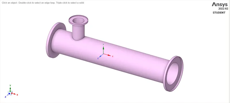
As we can see above figure is the Solid model, since we are interested in performing Fluid Flow analysis through geometry, hence we have extracted fluid volume from the Geometry. Space claim provides lots of options to extract Geometry. Go to prepare a menu and click on volume extract. Switch to edge selection and select three outer edges and click on the green check button.
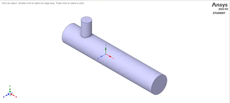
Hide solid by unchecking it from the structure menu to see the volume, which we have extracted We have used option Suppress for Physics to make sure that the solid component of geometry not to be involved in the Mesh generation process. So, Suppress the solid by clicking on the option suppress for physics.
Mesh Generation:
Meshing is the next step after the geometry clan up. Before mesh, we give boundary conditions to the body and we create the mesh. The boundary names inlet_x, inlet_y, outlet, and wall are defined using the named selection option.
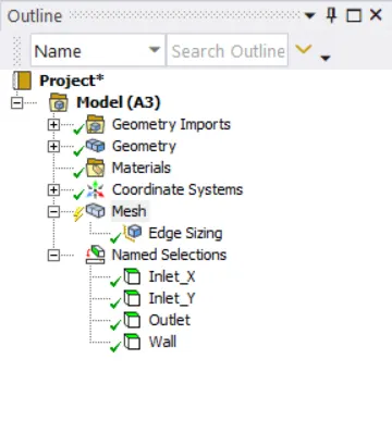
We have refined the mesh by an element size = 3mm and kept the rest of it default. After generating the mesh, the number of nodes and elements is investigated using the statistics option.
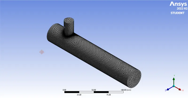
To get the converged results we need a good quality mesh with good quality mesh elements. Then the mesh quality is checked by choosing the mesh metric option in the quality section.
Here below we can see the quality of mesh elements in mesh matric.
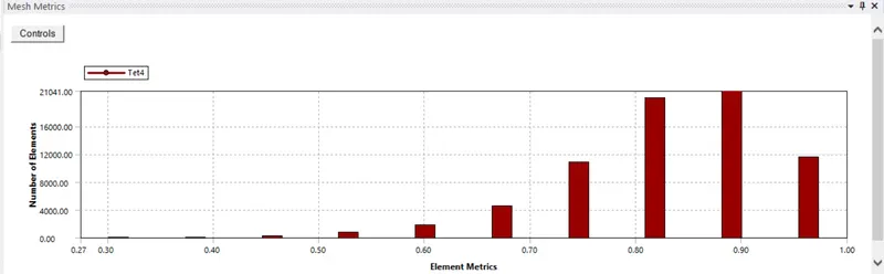
The element quality should not be less than 5%. In our case minimum mesh quality is 30%, so we can move ahead with this mesh for further study.
Setup:
Short TEE (MR=2 & Inlet Hot Velocity=3m/s)
| Solver Type | Pressure Based |
| Velocity Formulation | Absolute |
| Time | Steady |
| Viscous Model | k-omega SST model |
| Material | Air |
|
Cell zones Volume_volume |
Fluid type: Air |
| Boundaries |
Inlet x (velocity inlet): Velocity Magnitude – 3m/s Temperature – 36 degrees c. Inlet y (velocity inlet): Velocity Magnitude – 6m/s Temperature – 19 degrees c. Outlet (Pressure outlet) Gauge Pressure – 0 pascals. Walls – Stationary walls |
The hybrid scheme is used for initialization and the no. of iterations 200 is set up and then click on calculate option.
Results:
Residuals Plot
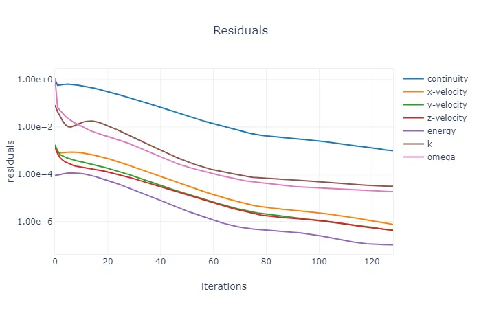
Iterations were taken to Converge: 129
Area weighted average temperature
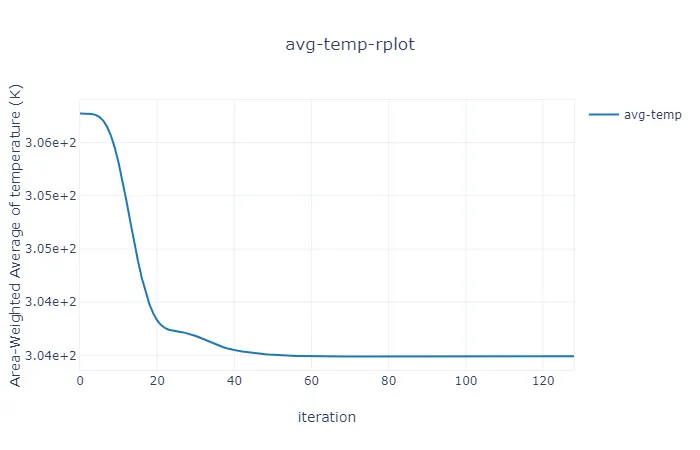
The above Plot shows that the average temperature of the Mixture at the Outlet is 303.5 Kelvin.
Standard Deviation
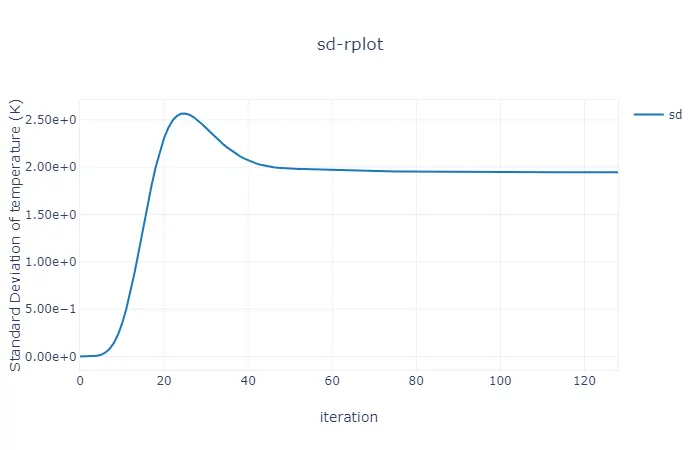
The above Plot shows that the standard deviation of temperature at the Outlet is 1.95 Kelvin.
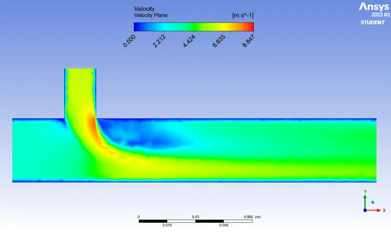
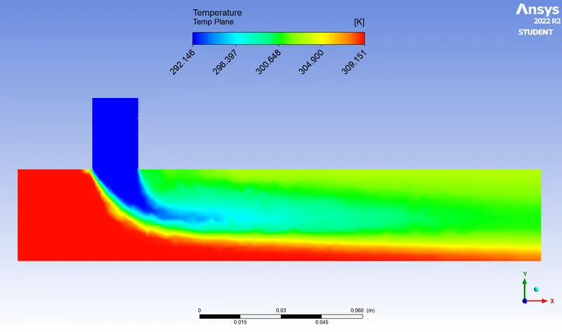
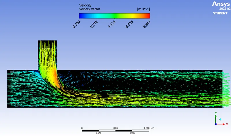
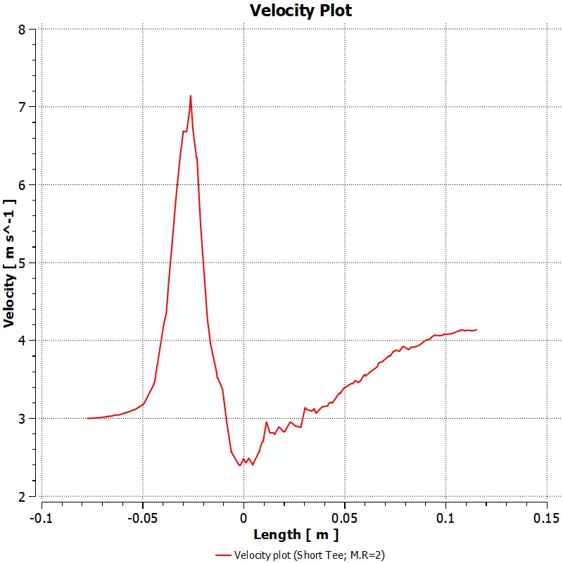
Contour Plots
1) Velocity Contour
2) Temperature Contour
3) Velocity Vector
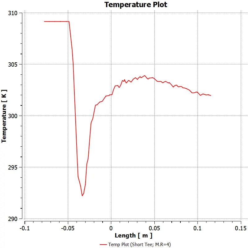
4) Velocity Chart
5) Temperature Chart
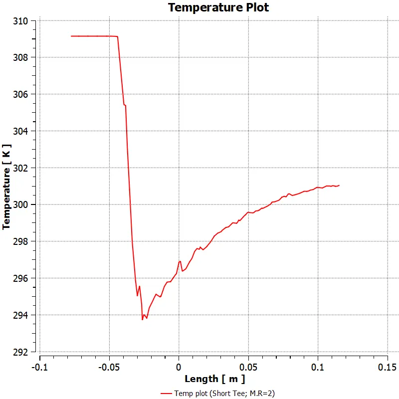
Subcase 2 ( Vh= 3m/s ; Vc= 12m/s) : Short mixing tee with a hot inlet velocity of 3m/s. Momentum ratio of 4
Geometry: Same as Subcase 1
Mesh Generation: Same as Subcase 1
Setup:
Short TEE (MR=4 & Inlet Hot Velocity=3m/s)
| Solver Type | Pressure Based |
| Velocity Formulation | Absolute |
| Time | Steady |
| Viscous Model | k-omega SST model |
| Material | Air |
|
Cell zones Volume_volume |
Fluid type: Air |
| Boundaries |
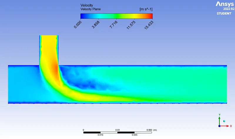
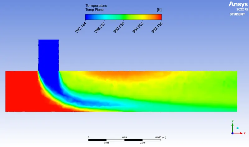
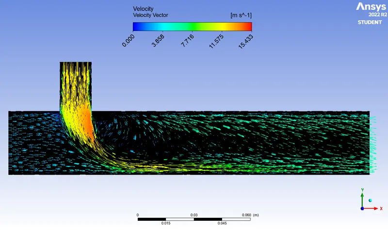
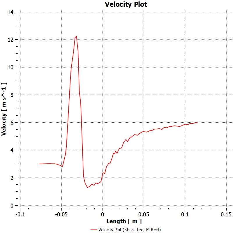
Inlet x (velocity inlet): Velocity Magnitude – 3m/s Temperature – 36 degrees c. Inlet y (velocity inlet): Velocity Magnitude – 12m/s Temperature – 19 degrees c. Outlet (Pressure outlet) Gauge Pressure – 0 pascals. Walls – Stationary walls |
The hybrid scheme is used for initialization and the no. of iterations 200 is set up and then click on calculate option.
Results:
Residuals Plot
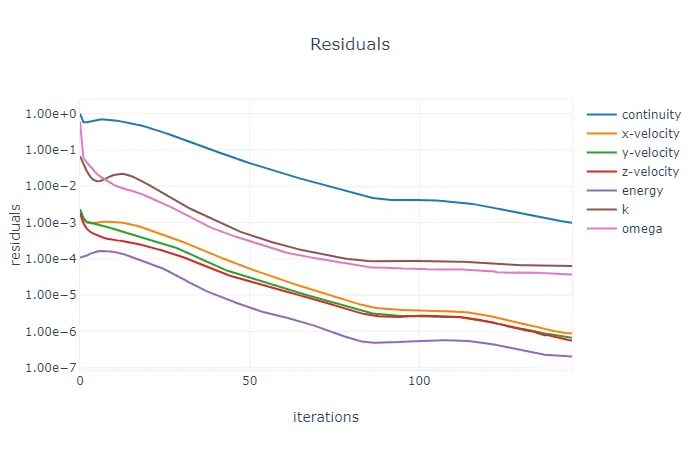
Iterations were taken to Converge: 146
Area weighted average temperature
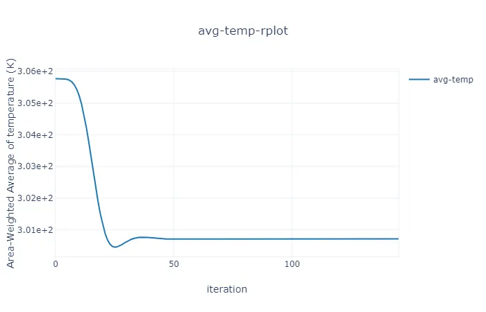
The above Plot shows that the average temperature of the Mixture at the Outlet is 300.70 Kelvin.
Standard Deviation
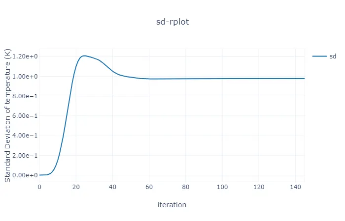
The above Plot shows that the standard deviation of temperature at the Outlet is 0.97 Kelvin.
Contour Plots
1) Velocity Contour
2) Temperature Contour
3) Velocity Vector
4) Velocity Chart
5) Temperature Chart
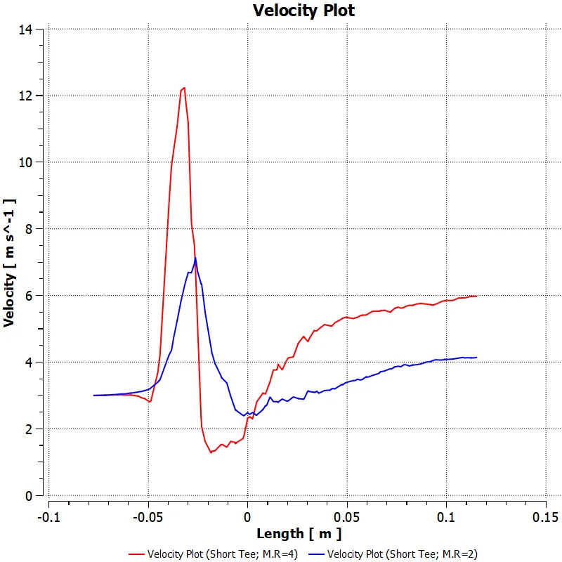
Summary:
Comparison between velocity plot for M.R=2 & M.R=4 of Short Tee
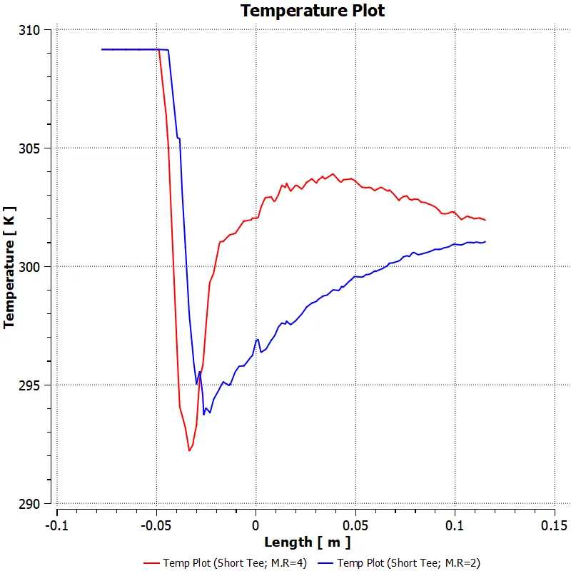
Comparison between temperature plot for M.R=2 & M.R=4 of Short Tee
Overall Comparision:
SHORT TEE
| M.R=2 | M.R=4 | |
| Viscous model | k-omega SST model | k-omega SST model |
| Cell count | 70,449 | 70,449 |
| Avg. Outlet Temperature | 303.5 K | 300.70 K |
| Standard Deviation | 1.95 K | 0.98 K |
| No of Iterations | 129 | 146 |
Conclusion:
1) For the k-omega SST model, the Standard Deviation of the Momentum Ratio 4 is lower than the Momentum Ratio 2. Hence the short tee with a momentum ratio of 4 has better mixing efficiency than the long tee with a momentum ratio of 2.
2) For the short tee, the Momentum Ratio 2 takes less number of iterations than the Momentum Ratio 2. Hence the short tee for the Momentum Ratio 2 is faster to Converge the solutions.
Case 2:
- Long mixing tee with a hot inlet velocity of 3m/s.
- Momentum ratio of 2, 4
In case 1 we are doing two different sub-cases one with a velocity of cold air at 6m/s and another with a velocity of cold air at 12m/s.
Subcase 1 ( Vh= 3m/s ; Vc= 6m/s) : Long mixing tee with a hot inlet velocity of 3m/s. Momentum ratio of 2
Geometry:
Import Short Tee geometry into Space claim, Space claim is CAD clean-up software that can be used to prepare CAD models for simulation setup. It could be for CFD or FEA.
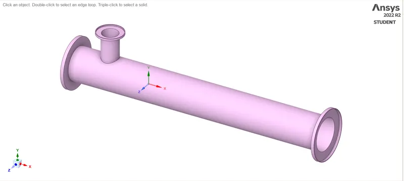
As we can see above figure is the Solid model, since we are interested in performing Fluid Flow analysis through geometry, hence we have extracted fluid volume from the Geometry. Space claim provides lots of options to extract Geometry. Go to prepare a menu and click on volume extract. Switch to edge selection and select three outer edges and click on the green check button.
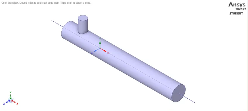
Hide solid by unchecking it from the structure menu to see the volume, which we have extracted We have used option Suppress for Physics to make sure that the solid component of geometry not to be involved in the Mesh generation process. So, Suppress the solid by clicking on the option suppress for physics.
Mesh Generation:
Meshing is the next step after the geometry clan up. Before mesh, we give boundary conditions to the body and we create the mesh. The boundary names inlet_x, inlet_y, outlet, and wall are defined using the named selection option.
We have refined the mesh by an element size = 3mm and kept the rest of it default. After generating the mesh, the number of nodes and elements is investigated using the statistics option.
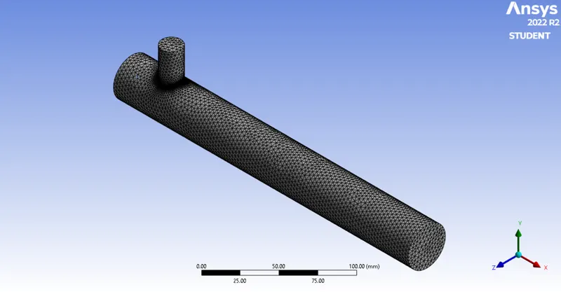
To get the converged results we need a good quality mesh with good quality mesh elements. Then the mesh quality is checked by choosing the mesh metric option in the quality section.
Here below we can see the quality of mesh elements in mesh matric.
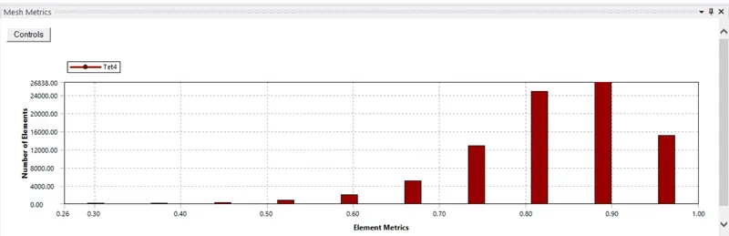
The element quality should not be less than 5%. In our case minimum mesh quality is 30%, so we can move ahead with this mesh for further study.
Setup:
Long TEE (MR=2 & Inlet Hot Velocity=3m/s)
| Solver Type | Pressure Based |
| Velocity Formulation | Absolute |
| Time | Steady |
| Viscous Model | k-omega SST model |
| Material | Air |
|
Cell zones Volume_volume |
Fluid type: Air |
| Boundaries |
Inlet x (velocity inlet): Velocity Magnitude – 3m/s Temperature – 36 degrees c. Inlet y (velocity inlet): Velocity Magnitude – 6m/s Temperature – 19 degrees c. Outlet (Pressure outlet) Gauge Pressure – 0 pascals. Walls – Stationary walls |
The hybrid scheme is used for initialization and the no. of iterations 200 is set up and then click on calculate option.
Results:
Residuals Plot
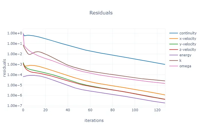
Iterations were taken to Converge: 128
Area weighted average temperature
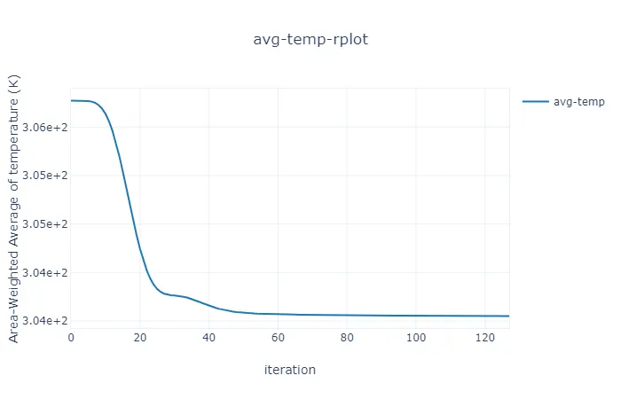
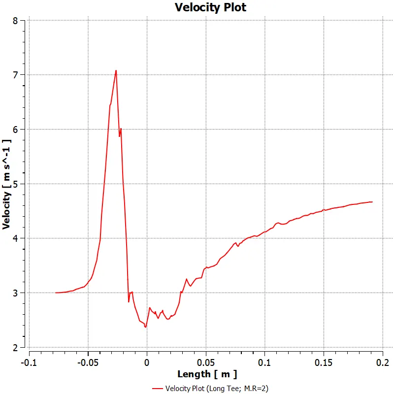
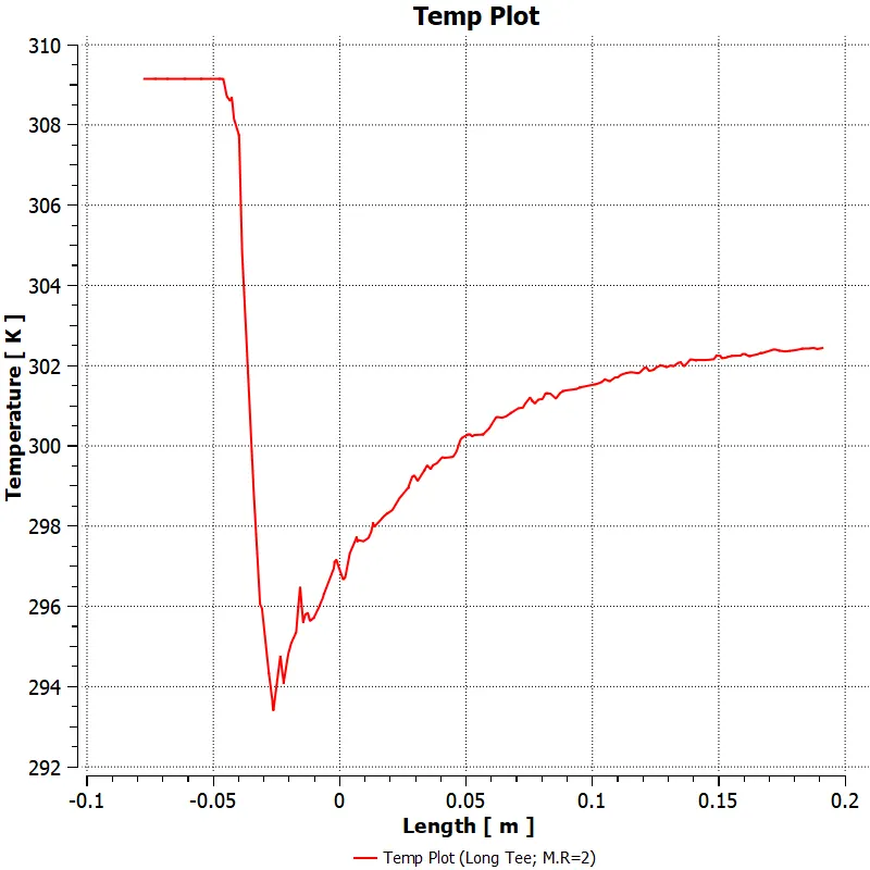
The above Plot shows that the average temperature of the Mixture at the Outlet is 303.5 Kelvin.
Standard Deviation
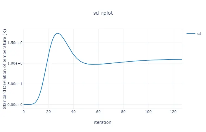
The above Plot shows that the standard deviation of temperature at the Outlet is 1.09 Kelvin.
Contour Plots
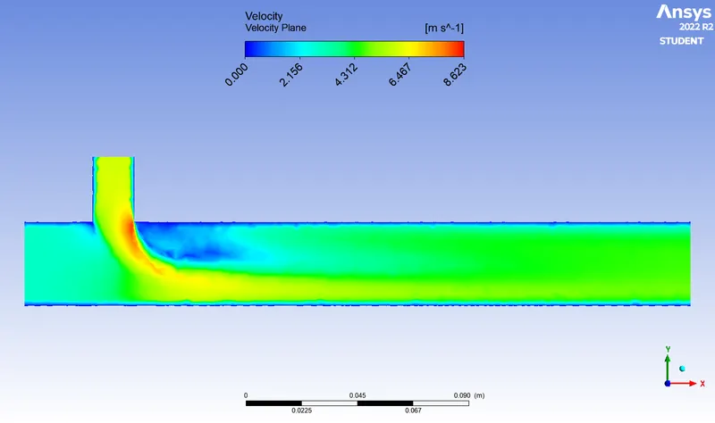
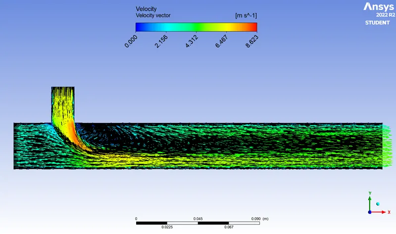
1) Velocity Contour
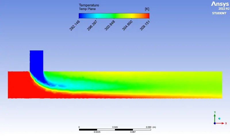
2) Temperature Contour
3) Velocity Vector
4) Velocity Chart
5) Temperature Chart
Subcase 2 ( Vh= 3m/s ; Vc= 12m/s) : Long mixing tee with a hot inlet velocity of 3m/s. Momentum ratio of 4
Geometry: Same as Subcase 1
Mesh Generation: Same as Subcase 1
Setup:
Long TEE (MR=4 & Inlet Hot Velocity=3m/s)
| Solver Type | Pressure Based |
| Velocity Formulation | Absolute |
| Time | Steady |
| Viscous Model | k-omega SST model |
| Material | Air |
|
Cell zones Volume_volume |
Fluid type: Air |
| Boundaries |
Inlet x (velocity inlet): Velocity Magnitude – 3m/s Temperature – 36 degrees c. Inlet y (velocity inlet): Velocity Magnitude – 12m/s Temperature – 19 degrees c. Outlet (Pressure outlet) Gauge Pressure – 0 pascals. Walls – Stationary walls |
The hybrid scheme is used for initialization and the no. of iterations 200 is set up and then click on calculate option.
Results:
Residuals Plot
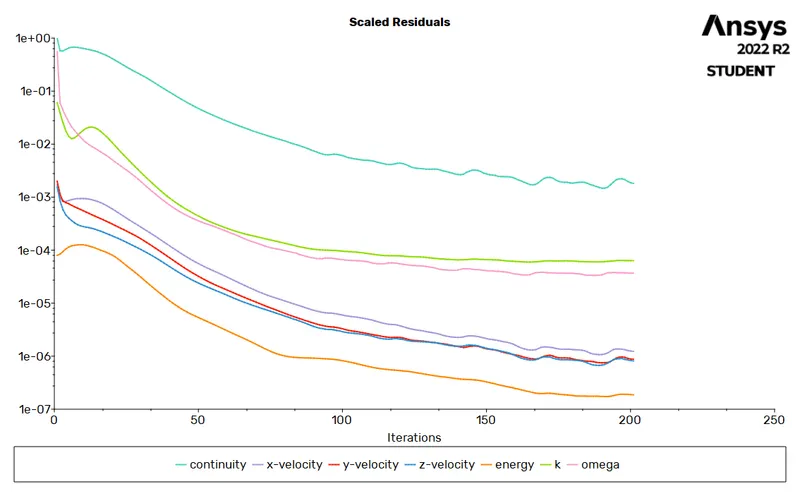
Iterations were taken to Converge: 100
Area weighted average temperature
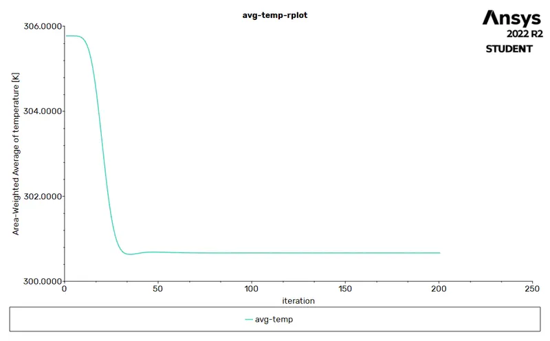
The above Plot shows that the average temperature of the Mixture at the Outlet is 300.67 Kelvin.
Standard Deviation
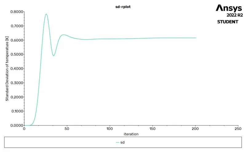
The above Plot shows that the standard deviation of temperature at the Outlet is 0.61 Kelvin.
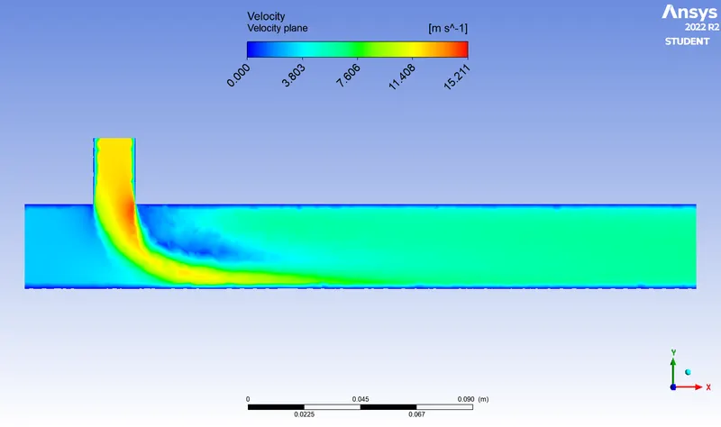
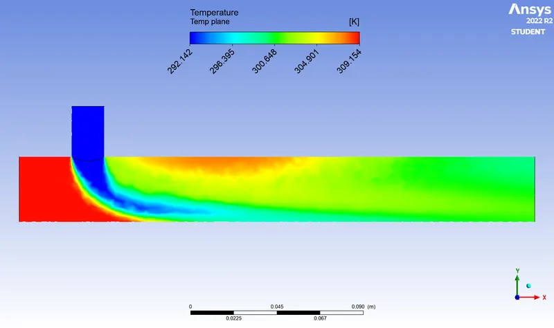
Contour Plots
1) Velocity Contour
2) Temperature Contour
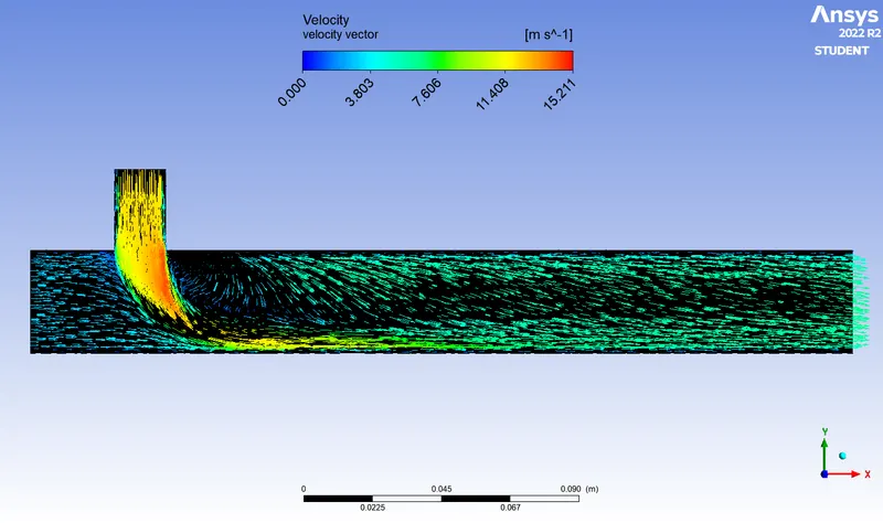
3) Velocity Vector
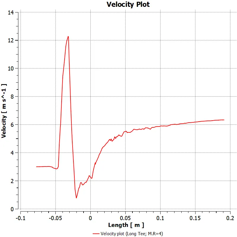
4) Velocity Chart
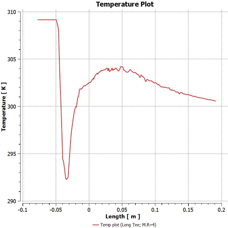
5) Temperature Chart
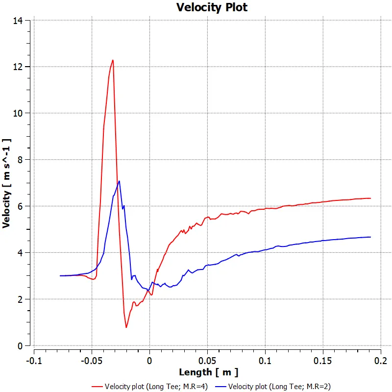
Comparison between velocity plot for M.R=2 & M.R=4 of Long Tee
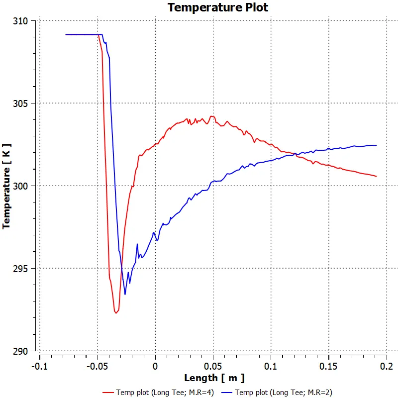
Comparison between temperature plot for M.R=2 & M.R=4 of Long Tee
Overall Comparision:
LONG TEE
| M.R=2 | M.R=4 | |
| Viscous model | k-omega SST model | k-omega SST model |
| Cell count | 86,966 | 86,966 |
| Avg. Outlet Temperature | 303.5 K | 300.66 K |
| Standard Deviation | 1.09 K | 0.61 K |
| No of Iterations | 128 | 100 |
Conclusion:
1) For the k-omega SST model, the Standard Deviation of the Momentum Ratio 4 is lower than the Momentum Ratio 2. Hence the long tee with a momentum ratio of 4 has better mixing efficiency than the long tee with a momentum ratio of 2.
2) For the long tee, the Momentum Ratio 4 takes less number of iterations than the Momentum Ratio 2. Hence the long tee for the Momentum Ratio 4 is faster to Converge the solutions.
OVERALL CONCLUSION:
- A short Tee is preferred rather than Long Tee because a Short tee has better mixing efficiency and low outlet Temperature than a long Tee.
- The Tee Mixing Effectiveness increases when the velocity of the cold inlet fluid increases. Hence Momentum Ratio of 4 has better effectiveness than 2.
- The outlet Temperature is also decreasing when the Momentum Ratio increases.
- Hence Momentum Ratio=4 is preferred over Momentum Ratio=2 due to the above-mentioned reasons.
Google Drive Link:
https://drive.google.com/drive/folders/1pjkaKTt78knBJN8kOVbjAInYw5abjyRF?usp=sharing