Week 1- Mixing Tee

Aim: To simulate mixing effectiveness of a hot and cold fluid mixing in a mixing tee using steady state simulation.

Objective: To simulate mixing effectiveness of hot and cold fluid in a mixing tee of different lengths and different momentum ratio and compare the results.

1. Case 1
   • Short mixing tee with a hot inlet velocity of 3m/s.
   • Momentum ratio of 2, 4.
2. Case 2
   • Long mixing tee with a hot inlet velocity of 3m/s.
   • Momentum ratio of 2, 4.

Momentum ratio = velocity at cold inlet / velocity at hot inlet

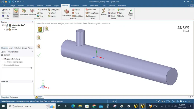
Procedure: In the Ansys Workbench Fluent solver is intialized and the given short tee model is loaded in the sapce claim.

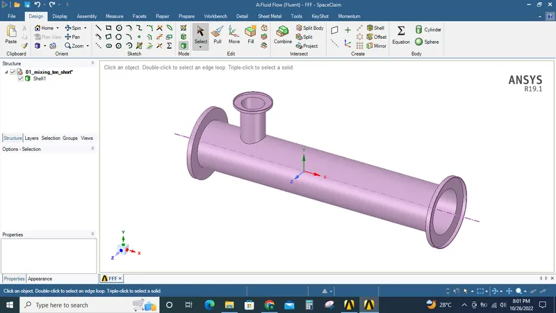
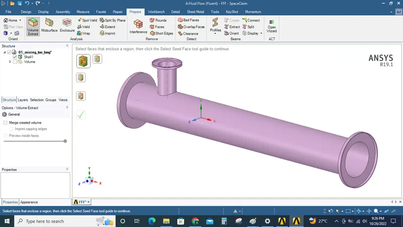
Using the volume extract tool under prepare ribbon tab, the volume is extracted.

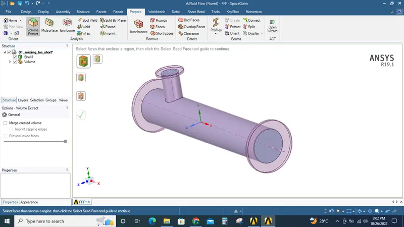
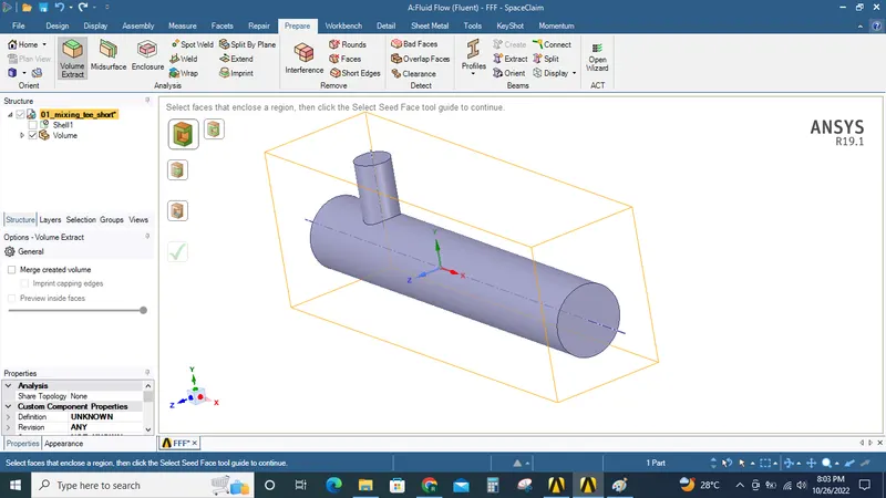
Once the desird volume is extarcted, with the help the struture tree the shell part of the model can be made hidden and aslo can be suppressed for simulations.

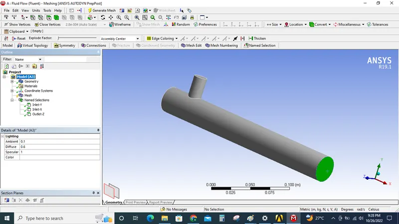
Now the mesh tool is intialized from Ansys window.

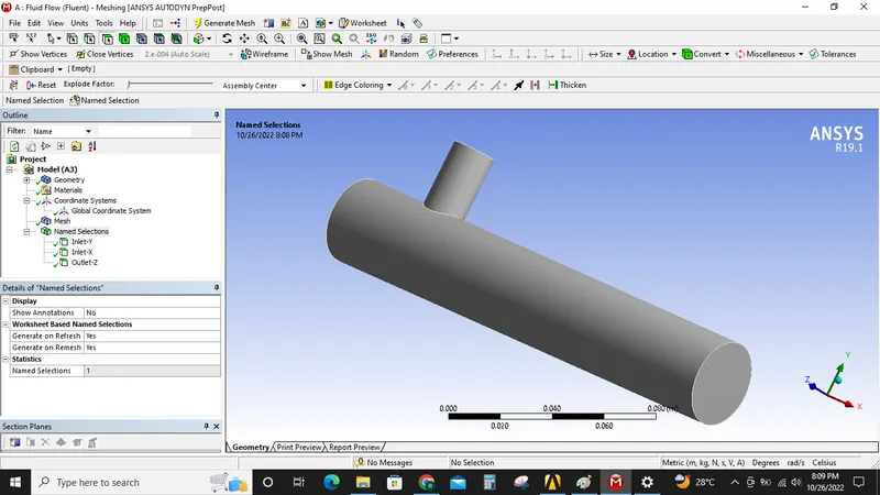
Here the inlets and the outlets are marked with the help of named selections.

Inlet-X
Inlet-Y

Outlet-Z

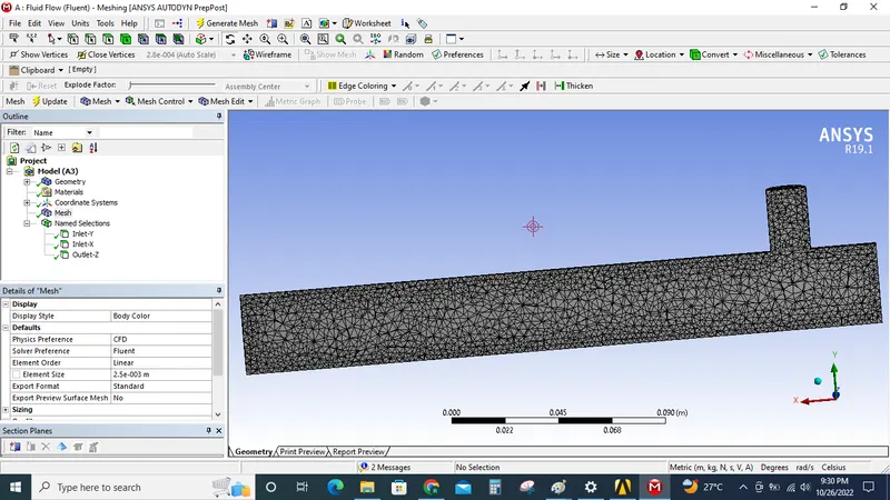
After this mesh is generated with default mesh parameters that has been provided by ansys

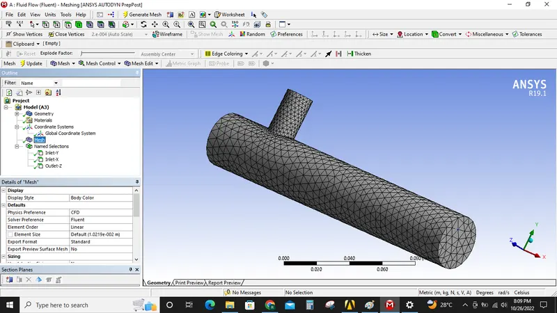
Default element size-1.0219e-002 M.

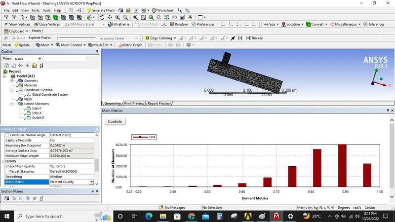
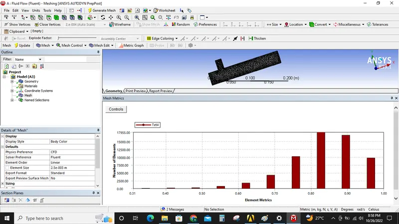
For this element size the element metrics are also within the allowed range.

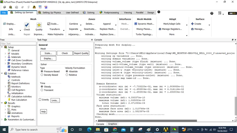
Now the mesh tool is closed and Fluent is opened in the Ansys project window.

Case1.1: Short tee with momentum ratio 2.

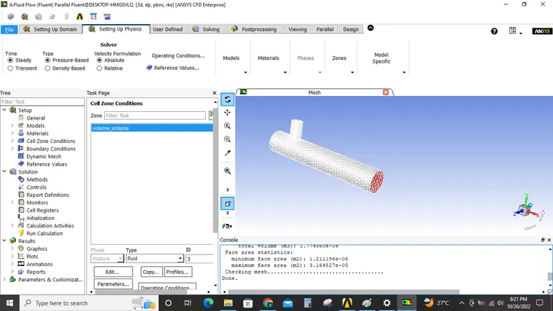
Once the model is loaded inside the Ansys fluent solver window, mesh qulaity check is done and found ok.

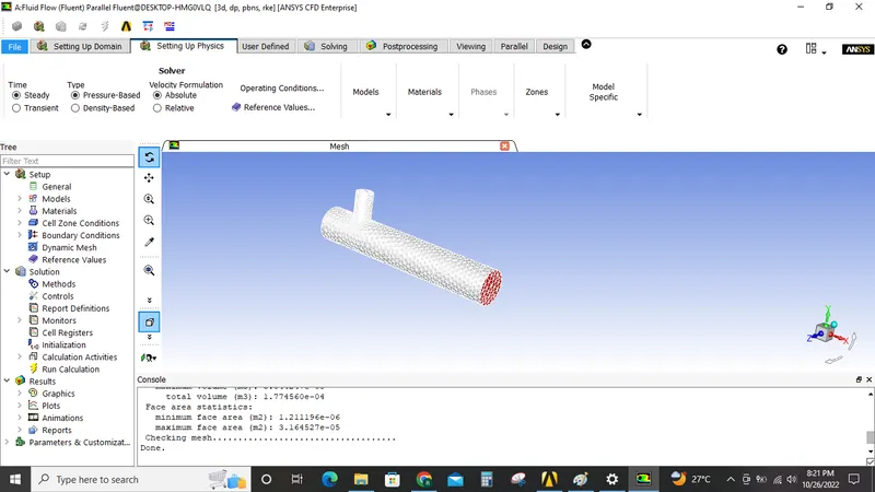
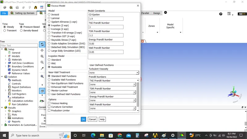
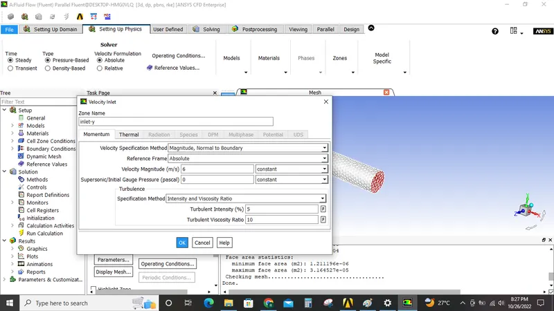
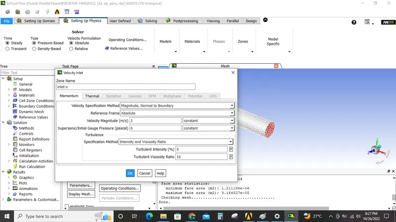
Under the setting up physics tab, steady state pressure based solver is selected and under the model group energy check box is selected since we are interested in the temperature.

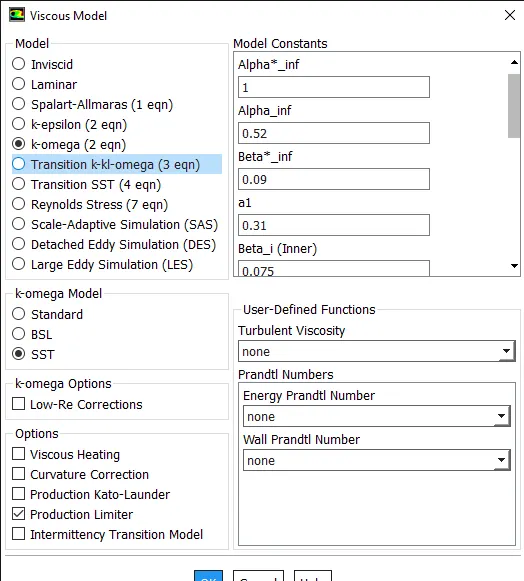
Realizable K- Epsilon model with standard wall function is selected for this simulation.

Material is set to air.

Under the boundary condition the inlet velocity along x axis is set to 3M/s with temperature 25° C.

Inlet velocity along Y axis is set to 6M/s with temperature 10°C.

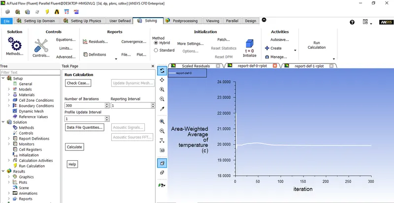
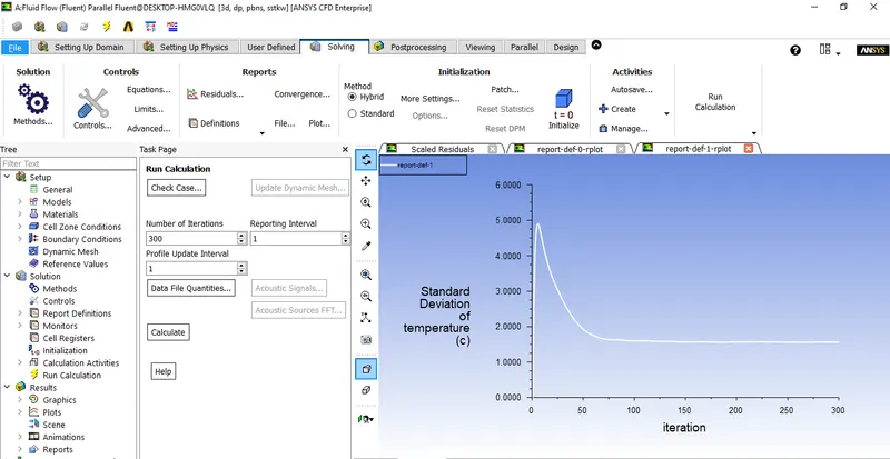
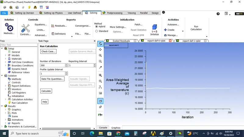
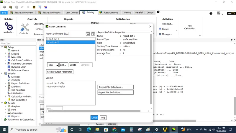
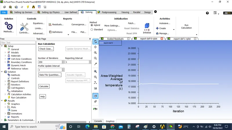
Under solving we have created Area wighted average report type at outlet for temperature and

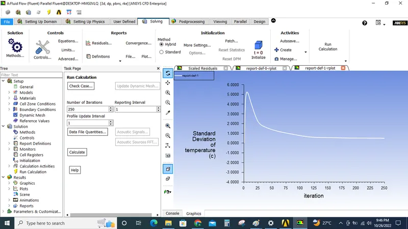
Standard deviation report type at outlet for temperature.

Outlet boundary condition is set to pressure based type.

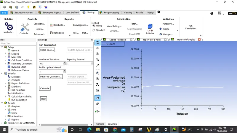
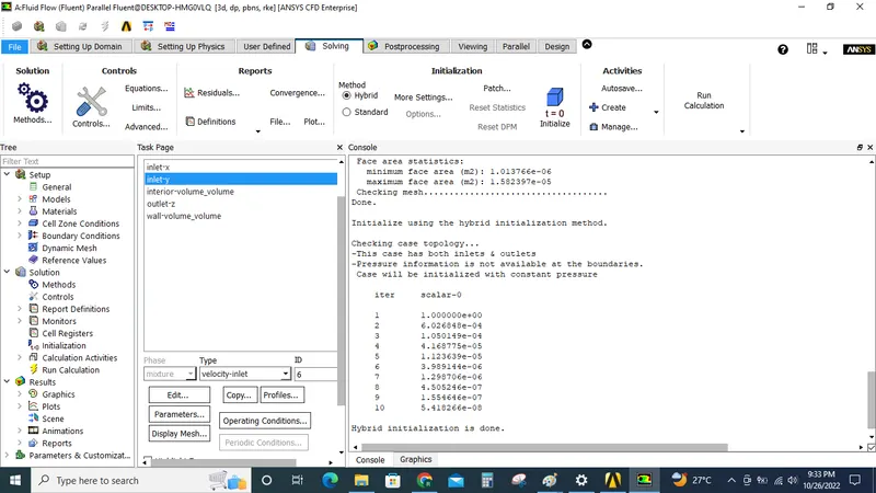
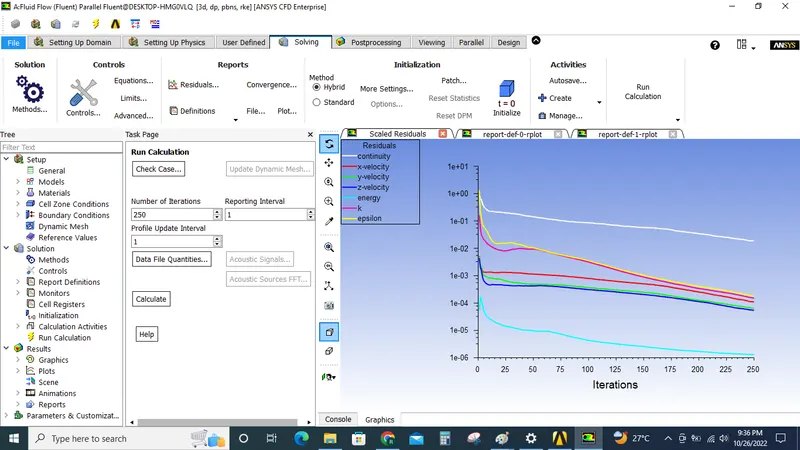
Once all boundary conditions are set the solution is Inizialized. Now the calculation is started with 250 iterations.

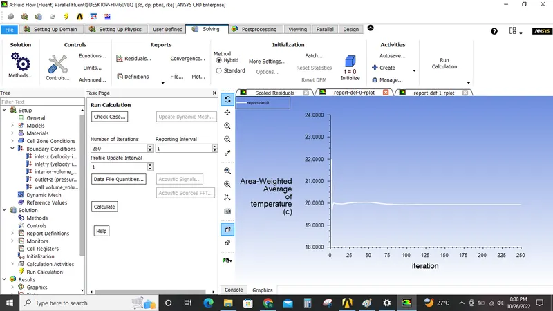
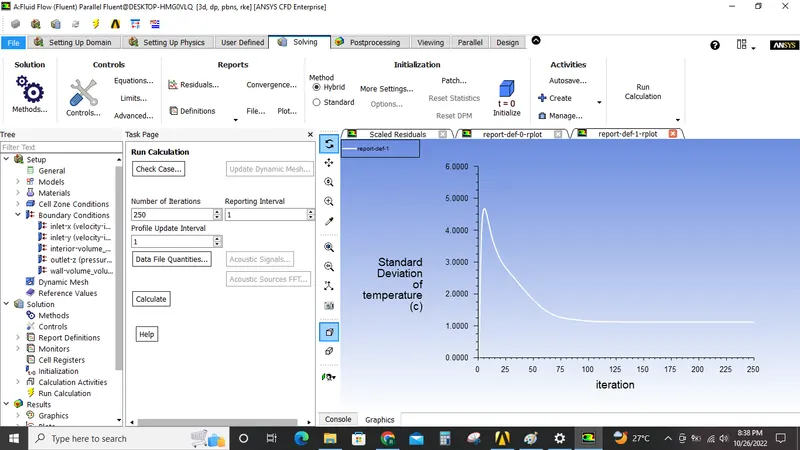
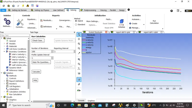
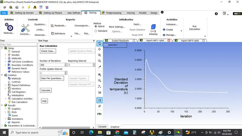
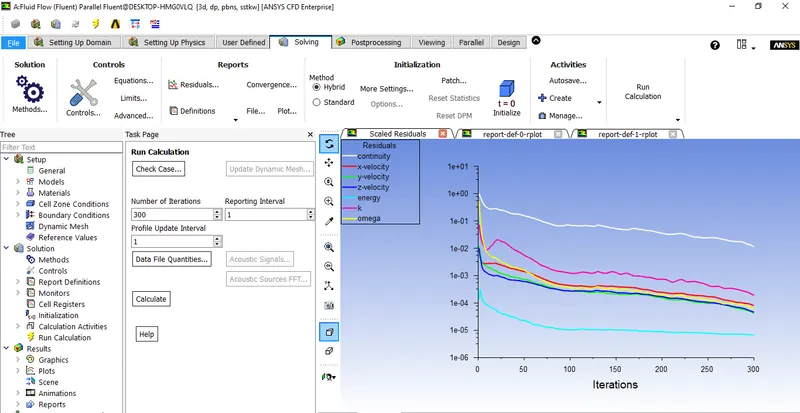
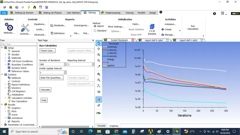
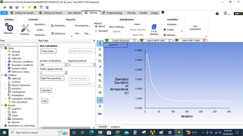
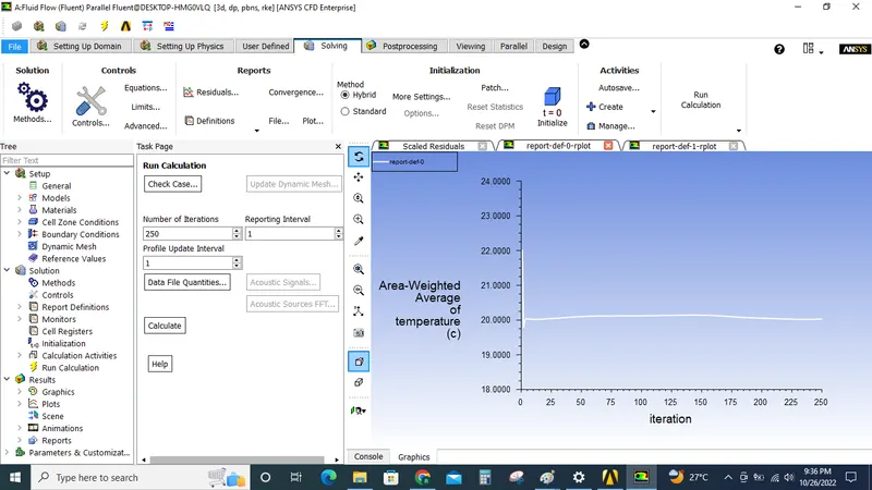
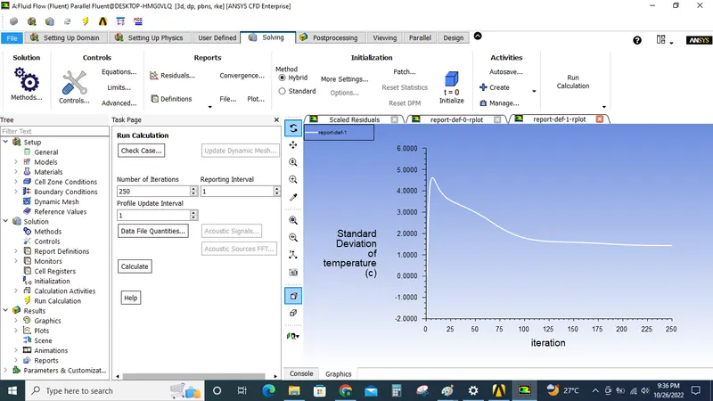
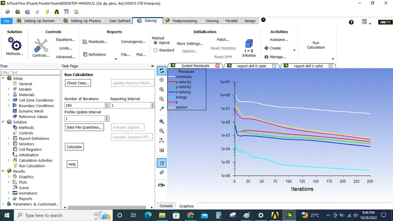
once the calculations are completed. It can be observed that the solution is converged as the residuals values go below 1e-03, also the values of the standard deviation and weighted average area became steady after 75 iterations.

Now Ansys fluent is closed and CFD post is opened in ansys project window.

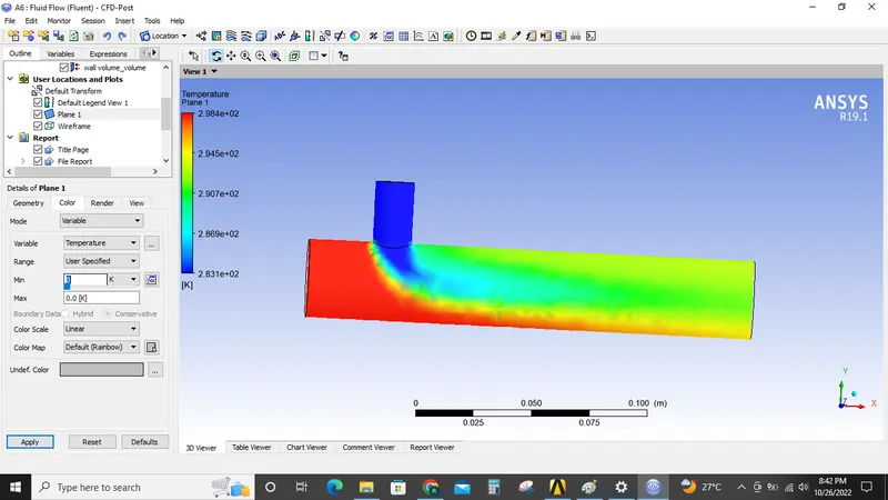
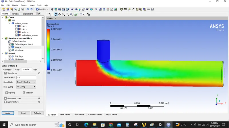
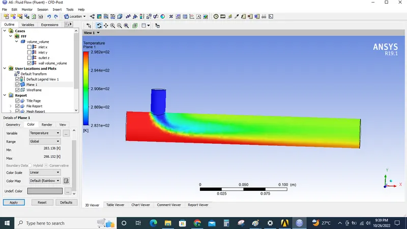
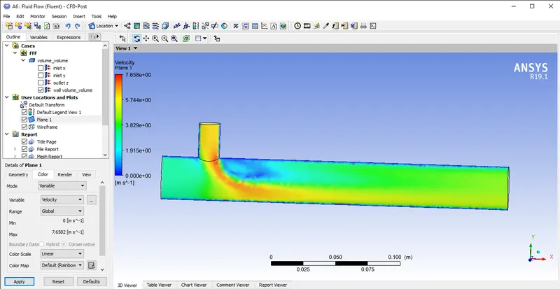
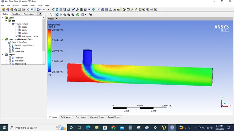
By inserting a plane and using temperature to render the plane we visualize the mixing contour plots of temperature and velocity.

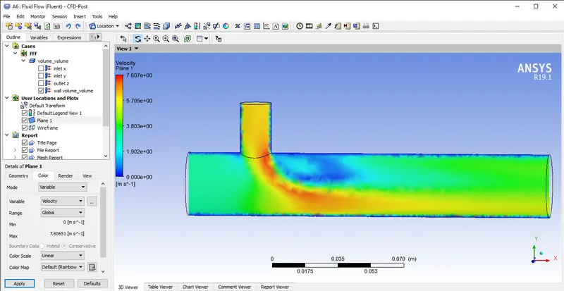
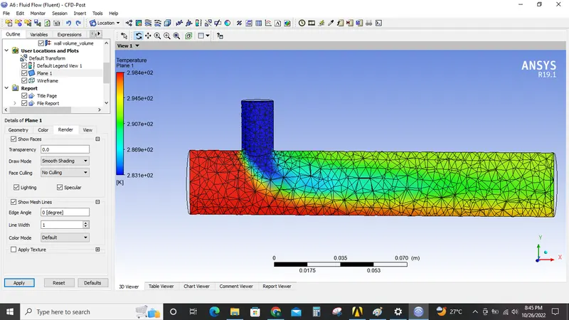
The contour plots look a bit diffused due to the mesh resolution.

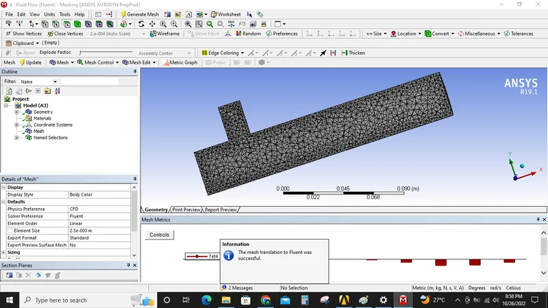
Now for the same case with the exact boundary conditions mesh independent study is done by changing the elements size to 2.5 MM. And the results are shown below.

\

t

Now the Temperatue contour plots look much better than the previous one.

now the same simulation is done using the K-omega SST method ans the results are shown below.

K-Epsilon Model:

The K-epsilon turbulence model is the most common model used in CFD to simulate turbulent flow conditions. It is a two-equation model that gives a description of turbulence by means of two transport equations (PDEs).

(K) - turbulent kinetic energy), (Epsilon)- Rate of dissipation of turbulent kinetic energy.

k-omega SST

Shear Stress Transport (SST) is a variant of the standard k–omega model. Combines the original Wilcox k-w model for use near walls and the standard k– Epsilon model away from walls using a blending function, and the eddy viscosity formulation is modified to account for the transport effects of the principle turbulent shear stress. SST is recommended for high accuracy boundary layer simulations.

Reason to use K-Epsilon Model:

k-omega model of turbulence is capable of solving turbulence parameters very close to boundary or wall region. If we are interested to capture the phenomenon in such region, we have to have very fine mesh near to the wall, so that Y+ value should be as small as possible. on the other hand, k- epsilon provides standard results. Since our interest is to study the mixing phenomena along the length, we are proceeding with Standard K-Epsilon model.

Case 1.2 Short tee with momentum ratio 4

Similar procedure is carried out as above to get the resukts that is shown below.

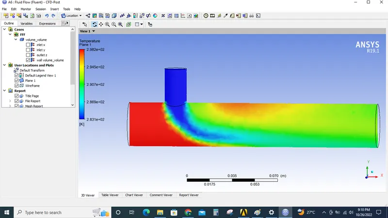
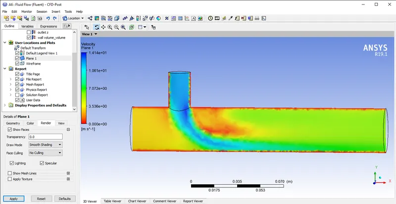
As we can see from the contour plots we are getting better mixing with high momentum ratio.

Case 2.1 Long tee with momentum ratio of 2.

The simulation is performed following the same procedure as above

Long tee

Inlet temperature along x axis-- 25°C and 3M/s

Inlet temperature along Y axis --10°C and 6 M/S

Case 2.1: Long tee with momentum ratio 4

Long tee

Inlet temperature along x axis-- 25°C and 3M/s

Inlet temperature along Y axis --10°C and 12 M/S

As we can see from the contour plots we are getting better mixing with high momentum ratio just like the short tee case. And the length of the tee does not make much difference in the end results.

		Mixing tee	Momentum ratio	Inlet temperature-X	Inlet temperature-Y	Element size	Cell count	Avg outlet temperature	No. of iterations for convergence
1	Case 1.1	Short	2	25°C	10°C	2.5 MM	61446	20.1°C	250
2	Case 1.2	Short	4	25°C	10°C	2.5 MM	61446	18.4°C	240
3	Case2.1	Long	2	25°C	10°C	2.5 MM	86848	20.1°C	180
4	Case2.2	Long	4	25°C	10°C	2.5 MM	86848	18.5°C	225

Conclusion:

Mesh size of 2.5 MM gives the best results.

Momentum ratio 4 gives better results than momentum ratio 2.