Week 1- Mixing Tee

OBJECTIVE:

• To set up steady-state simulations to compare the mixing effectiveness when the hot inlet temperature is 36⁰C & the Cold inlet is 19⁰C.
• Using the k-epsilon and k-omega SST model for the first case and based on our judgment we will use the more suitable model for further cases.
• Understand the effect of length of pipe and momentum ratio of velocity for mixing of air by using two different types of pipe i.e. short pipe and long pipe.

We have to consider two cases for Simulations

• Case 1: Short Mixing tee with a hot inlet velocity of 3 m/s with Momentum Ratio (MR)=2.
• Case 2: Short Mixing tee with a hot inlet velocity of 3 m/s with Momentum Ratio (MR)=4.
• Case 3: Long Mixing tee with a hot inlet velocity of 3 m/s with Momentum Ratio (MR)=2.
• Case 4: Long Mixing tee with a hot inlet velocity of 3 m/s with Momentum Ratio (MR)=4.

INTRODUCTION:

Computational fluid dynamics (CFD) is a branch of fluid mechanics that uses numerical analysis and data structures to analyze and solve problems that involve fluid flows. Computers are used to perform the calculations required to simulate the free-stream flow of the fluid, and the interaction of the fluid (liquids and gases) with surfaces defined by boundary conditions.

CFD is applied to a wide range of research and engineering problems in many fields of study and industries, including aerodynamics and aerospace analysis, hypersonics, weather simulation, natural science and environmental engineering, industrial system design and analysis, biological engineering, fluid flows, and heat transfer, engine and combustion analysis, and visual effects for the film. Although CFD has widespread real-world applications across many industries, it is difficult to master, hence, many companies overcome this knowledge barrier by engaging CFD

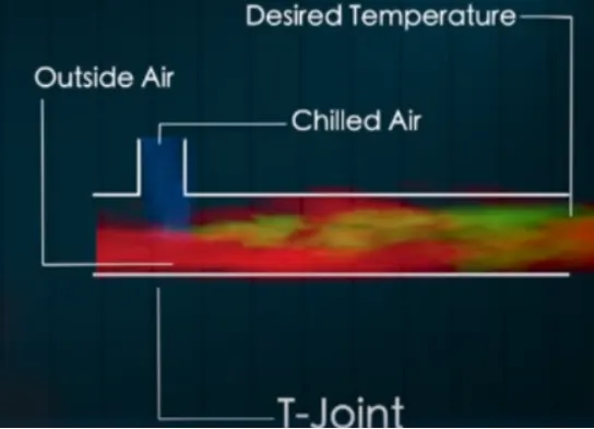
The function of the mixing Tee is to provide proper mixing of hot and cold Air to get the desired result at the outlet.

GEOMETRY:

SHORT TEE:

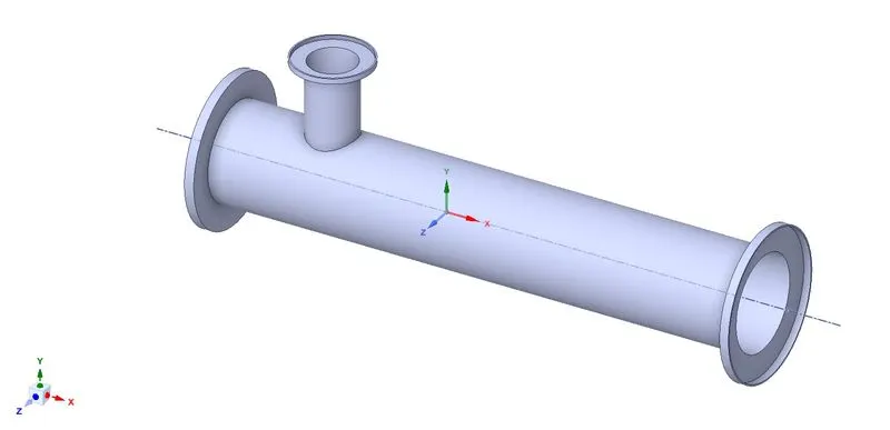
First we upload the Geometry in SpaceClaim and we have to clean the body that is taken into consideration for simulation and remove the unwanted geometry using Volume extract method.

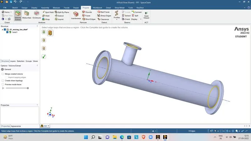
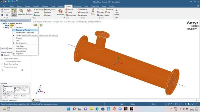
Extract the Volume:

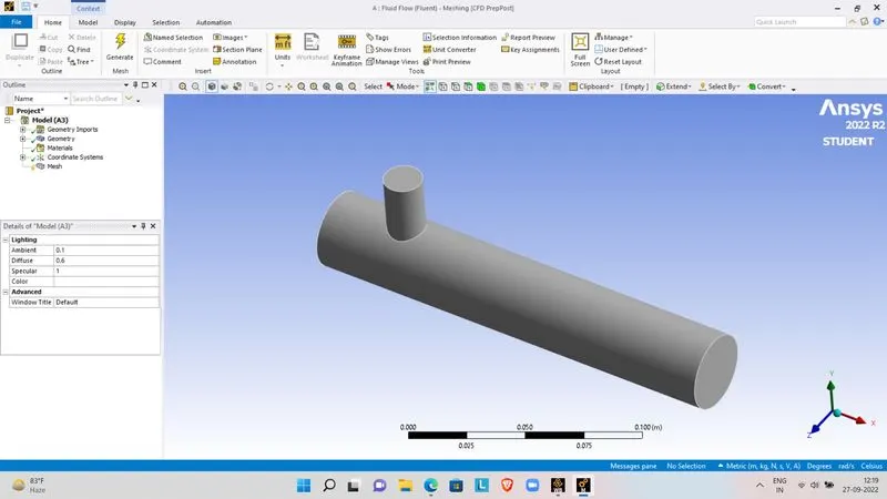
Select each face and name using named selection method.

Named Selections:

• Inlet X: Inlet along the x direction.
• Inlet Y: Inlet along the Y direction.
• Outlet: Outlet along the x direction.
• Wall: The entire boundary of the extracted volume is selected

MESH GENERATION:

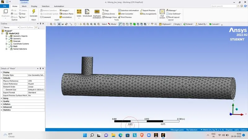
• Size:0.010219m
• Node: 2804
• Element: 12608

After the Meshing is done, we check the Mesh quality in mesh matrics. We get a good mesh when the element quality of the mesh matrics is more than 30%.

SETUPS	CASE 1:SHORT TEE (MR=2 AND HOT INLET VELOCITY = 3m/s)
	CASE 1.1: K-EPSILON	CASE 1.2: K-OMEGA
SOLVER TYPE	Pressure based	Pressure based
VELOCITY FORMULATION	Absolute	Absolute
TIME	Steady	Steady
VISCOUS MODEL	Realizable K-epsilon with standard wall function	K-omega SST model
MATERIAL	Air	Air
CELL ZONES	Fluid type : air	Fluid type : air
BOUNDARIES	· Inlet_x (velocity inlet) Velocity magnitude 3m/s Temperature - 360c · Inlet_y (velocity inlet) Velocity magnitude 6m/s Temperature – 190c · Outlet (pressure outlet) Gauge pressure – 0 pa · Walls – stationary walls	· Inlet_x (velocity inlet) Velocity magnitude 3m/s Temperature - 360c · Inlet_y (velocity inlet) Velocity magnitude 6m/s Temperature – 190c · Outlet (pressure outlet) Gauge pressure – 0 pa · Walls – stationary walls

The hybrid scheme is used for initialization and the no. of iterations are setup and then click on calculate option.

RESULTS:

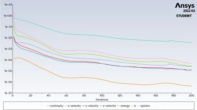
RESIDUAL PLOT:

CASE 1.1: K-EPSILON MODEL:

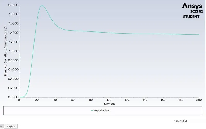
STANDARD DEVIATION:

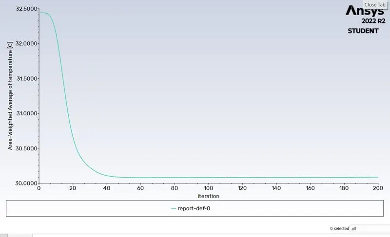
AREA WEIGHTED AVERAGE OF TEMPERATURE:

CONTOUR PLOT:

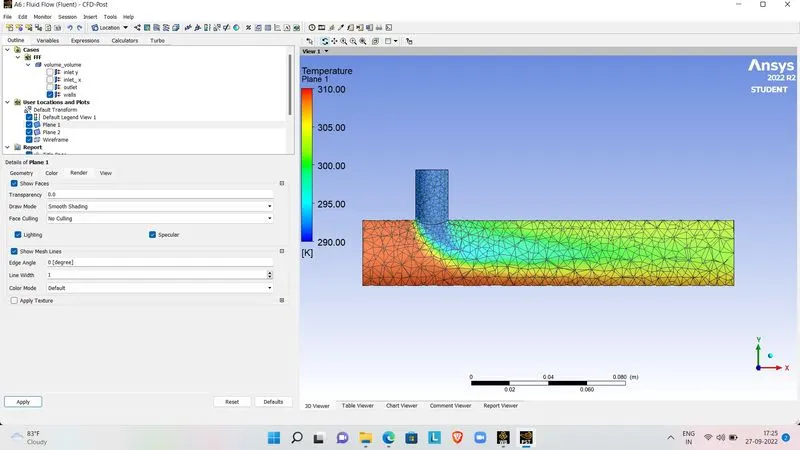
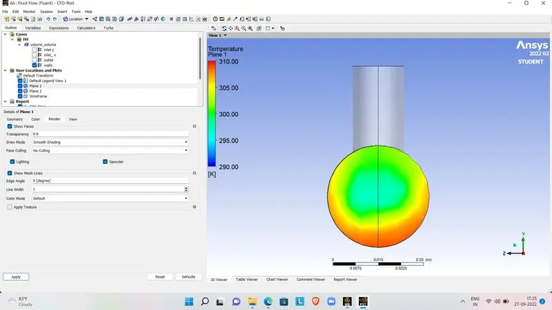
TEMPERATURE CONTOUR:

ALONG THE PLANE:

ACROSS THE PLANE:

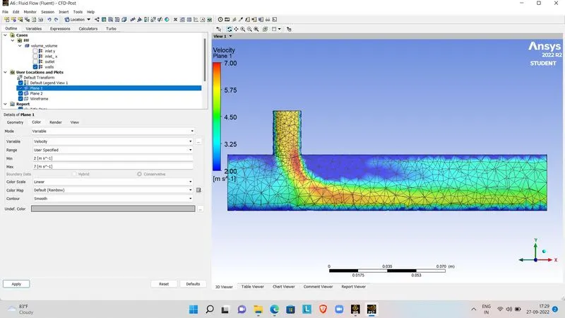
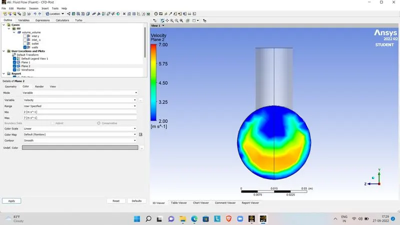
VELOCITY CONTOUR:

ALONG THE PLANE:

ACROSS THE PLANE

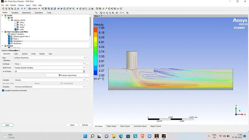
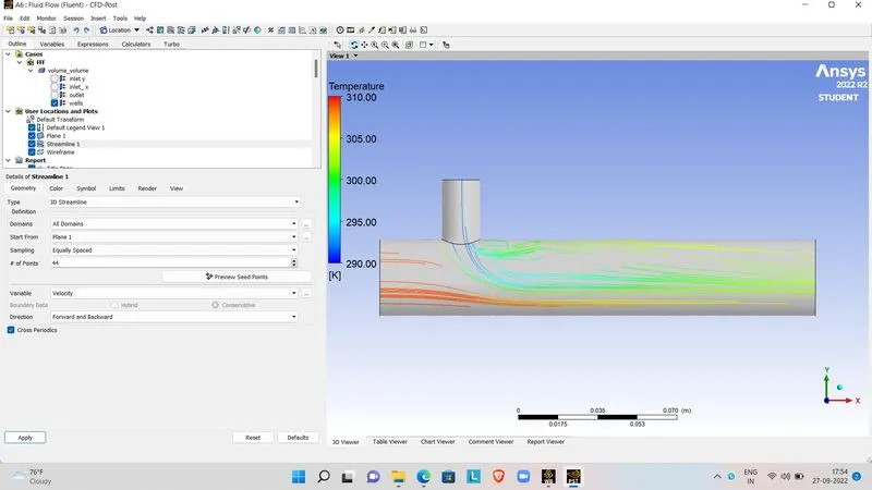
STREAMLINE PLOT:

VELOCITY PLOT:

TEMPERATURE PLOT:

CASE 1.2: K-OMEGA MODEL:

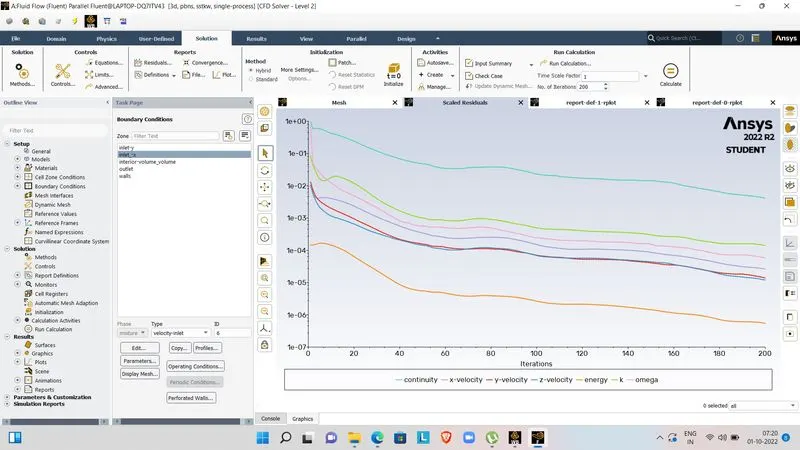
RESIDUAL PLOT:

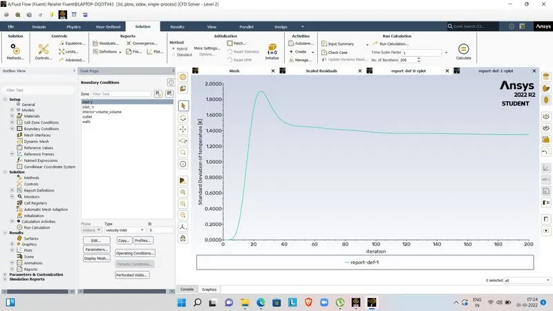
STANDARD DEVIATION:

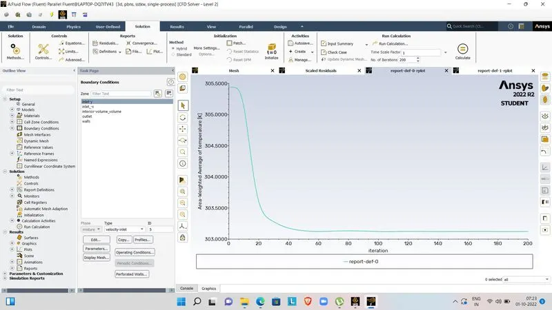
AREA WEIGHTED AVERAGE TEMPERATURE:

CONTOUR PLOT:

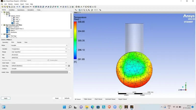
TEMPERATURE PLOT:

ALONG THE PLANE:

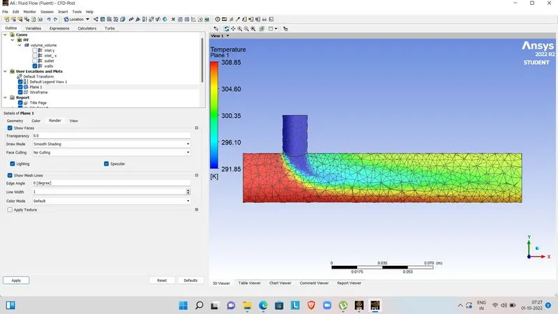
ACROSS THE PLANE:

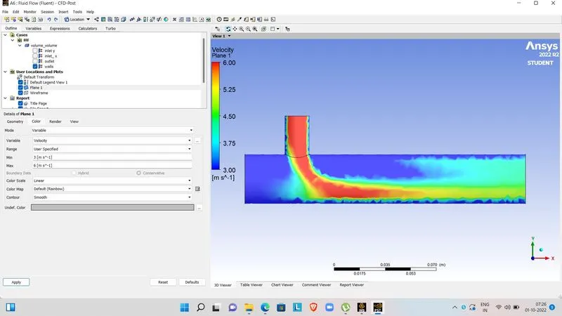
VELOCITY PLOT:

ALONG THE PLANE:

ACROSS THE PLANE:

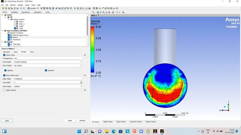
STREAMLINE PLOT:

VELOCITY PLOT:

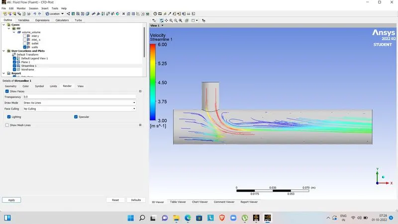
TEMPERATURE PLOT:

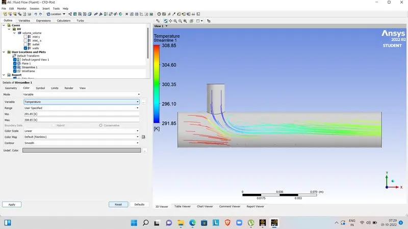
OBSERVATION FROM ABOVE RESULTS:

SHORT TEE (MR = 2)
	K- EPSILON	K-OMEGA
AVERAGE OUTLET TEMPERATURE [C]	30.32	30.34
STANDARD DEVIATION	1.51	1.55
NO OF ITERATIONS	150	160

CASE 2:

• Short mixing Tee with a hot inlet velocity of 3m/s
• Momentum ratio of 4

SETUPS	SHORT TEE (MR=2 AND HOT INLET VELOCITY = 3m/s)
	CASE 2.1: K-EPSILON	CASE 2.2: K-OMEGA
SOLVER TYPE	Pressure based	Pressure based
VELOCITY FORMULATION	Absolute	Absolute
TIME	Steady	Steady
VISCOUS MODEL	Realizable K-epsilon with standard wall function	K-omega SST model
MATERIAL	Air	Air
CELL ZONES	Fluid type : air	Fluid type : air
BOUNDARIES	· Inlet_x (velocity inlet) Velocity magnitude 3m/s Temperature - 360c · Inlet_y (velocity inlet) Velocity magnitude 12m/s Temperature – 190c · Outlet (pressure outlet) Gauge pressure – 0 pa · Walls – stationary walls	· Inlet_x (velocity inlet) Velocity magnitude 3m/s Temperature - 360c · Inlet_y (velocity inlet) Velocity magnitude 12m/s Temperature – 190c · Outlet (pressure outlet) Gauge pressure – 0 pa · Walls – stationary walls

The hybrid scheme is used for initialization and the no. of iterations are setup and then click on calculate option.

RESULTS:

CASE 2.1: K-EPSILON

RESIDUAL PLOT:

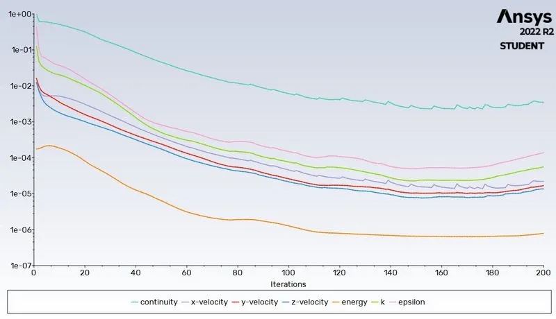
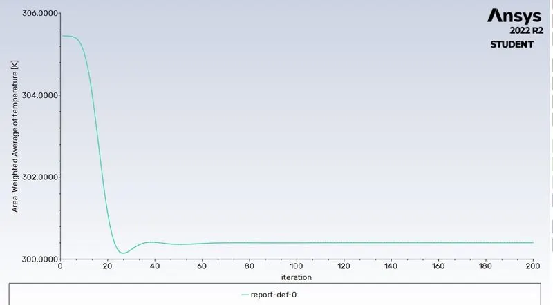
AREA WEIGHTED AVERAGE TEMPERATURE:

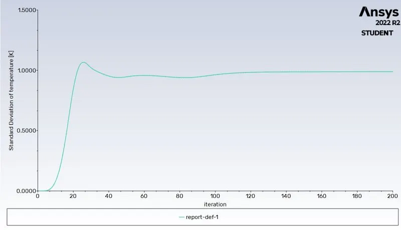
STANDARD DEVIATION:

CONTOUR PLOTS:

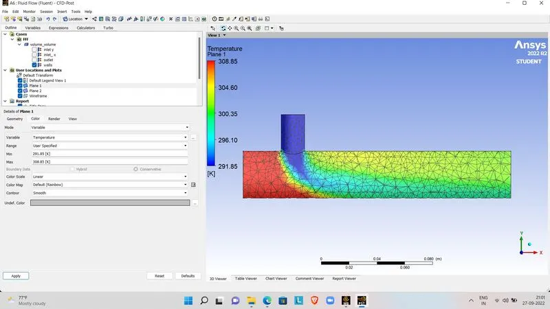
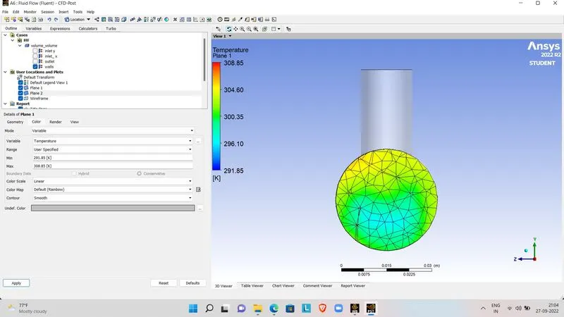
TEMPERATURE PLOT:

ALONG THE PLANE:

ACROSS THE PLANE:

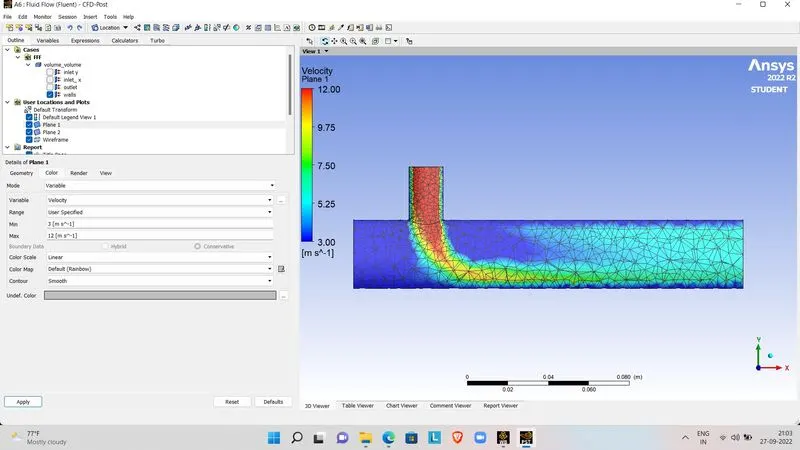
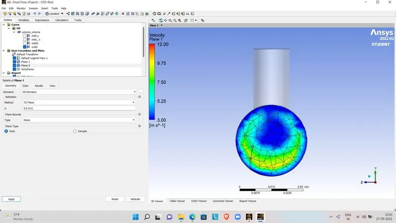
VELOCITY PLOT:

ALONG THE PLANE:

ACROSS THE PLANE:

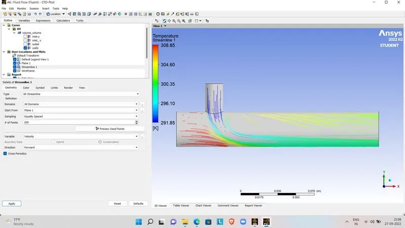
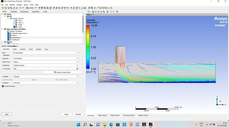
STREAMLINE PLOT:

TEMPERATURE PLOT:

VELOCITY PLOT:

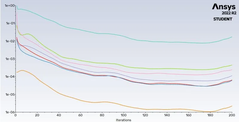
CASE 2.1 K-OMEGA SST MODEL

RESIDUAL PLOT:

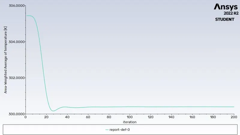
AREA WEIGHTED AVERAGE TEMPERATURE :

STANDARD DEVIATION:

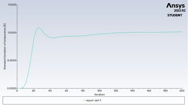
CONTOUR PLOTS:

TEMPERATURE PLOT:

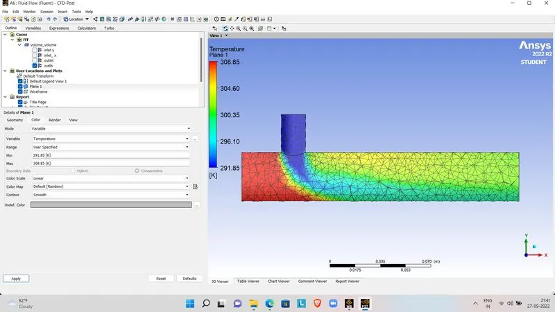
VELOCITY PLOT:

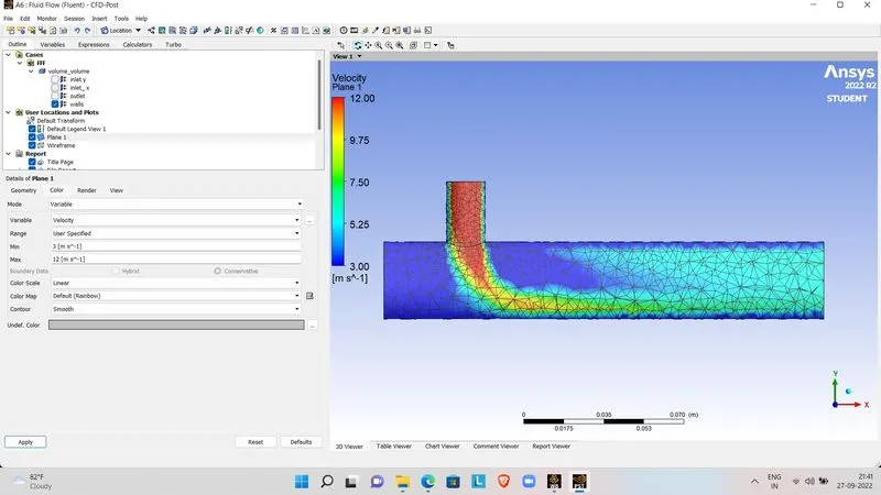
SUMMARY FROM ABOVE OBSERVATION:

SHORT TEE (MR = 4)
K-EPSILON	K-EPSILON	K-OMEGA
AVERAGE OUTLET TEMPERATURE [C]	27.34	27.3
STANDARD DEVIATION	1.1	1.2
NO OF ITERATIONS	140	150

ANALYTICAL SOLUTION:

MOMENTUM RATIO 2:

• Mass of hot fluid (m_h) = rho*a*V_h = (1.225*897.79*3)/1000000=0.00329937825
• Mass of cold fluid (m_c) = rho*a*V_c = (1.225*224.88*6)/1000000 = 0.001652868
• Temperature of mixture (T_mixture) = (m_h*T_h + m_c*T_c)/(m_c + m_h) = 30.32⁰c

MOMENTUM RATIO 4:

• Mass of hot fluid (m_h) = rho*a*V_h = (1.225*897.79*3)/1000000=0.00329937825
• Mass of cold fluid (m_c) = rho*a*V_c = (1.225*224.86*12)/1000000=0.003305736
• Temperature of mixture (T_mixture) = (m_h*T_h + m_c*T_c)/(m_c + m_h) = 27.34⁰c

CONCLUSION:

• On comparing both models with the analytical solution we got nearly the same results.
• No. of iterations taken to converge is less for Realisable K-epsilon model than K-omega SST model.
• The standard deviation of k-epsilon model is less than k-omega model which shows better mixing efficiency in k-epsilon model.

So based on the above observations the K-epsilon turbulence model is predicting the results accurately in less no. of iterations. So we can use realisable k-epsilon model for case 3

CASE 3: LONG TEE HOT INLET VELOCITY 3m/s MR=2

GEOMETRY SETUP:

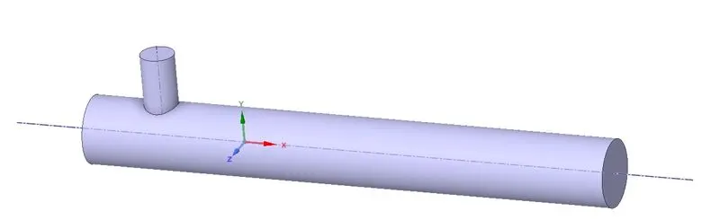
First, we have to upload the geometry of the long mixing tee in Spaceclaim. After uploading we have to select the edges and extract the volume. After extracting, we need to suppress the unwanted components, and suppress the physics.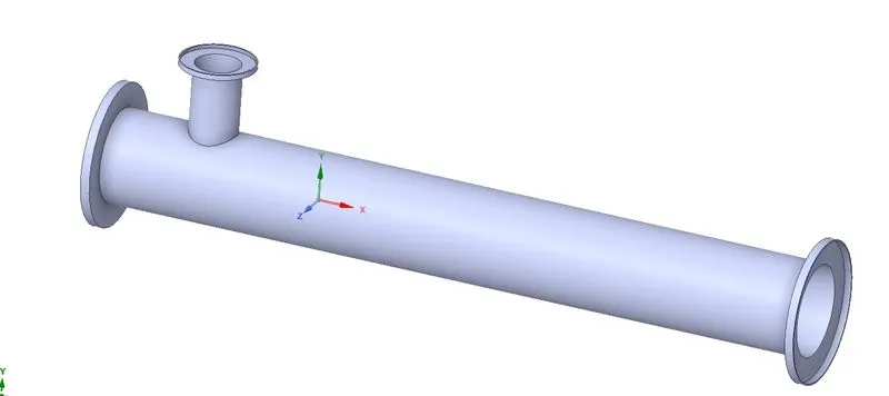

MESH GENERATION:

SETUPS	LONG TEE (MR=2 AND HOT INLET VELOCITY 3m/s)
	K-EPSILON
SOLVER TYPE	Pressure based
VELOCITY FORMULATION	Absolute
TIME	Steady
VISCOUS MODEL	Realizable K-epsilon with standard wall function
MATERIAL	Air
CELL ZONES	Fluid type : air
BOUNDARIES	· Inlet_x (velocity inlet) Velocity magnitude 3m/s Temperature - 360c · Inlet_y (velocity inlet) Velocity magnitude 6m/s Temperature – 190c · Outlet (pressure outlet) Gauge pressure – 0 pa · Walls – stationary walls

The hybrid scheme is used for initialization and the no. of iterations are setup and then click on calculate option.

RESULTS:

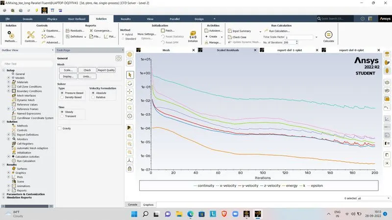
RESIDUAL PLOT:

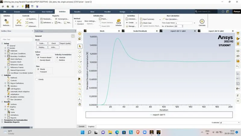
STANDARD DEVIATION:

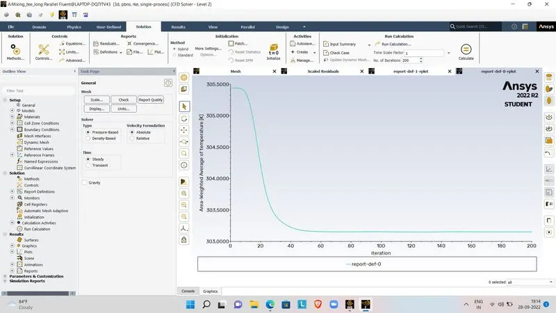
AREA WEIGHTED AVERAGE TEMPERATURE:

CASE 4: LONG MIXING TEE , HOT INLET VELOCITY=3m/s , MR=4

RESULTS:

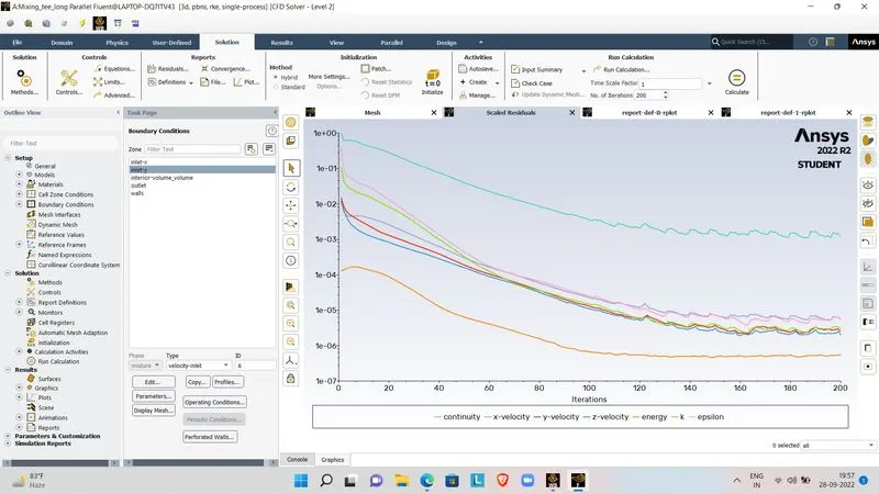
RESIDUAL PLOT:

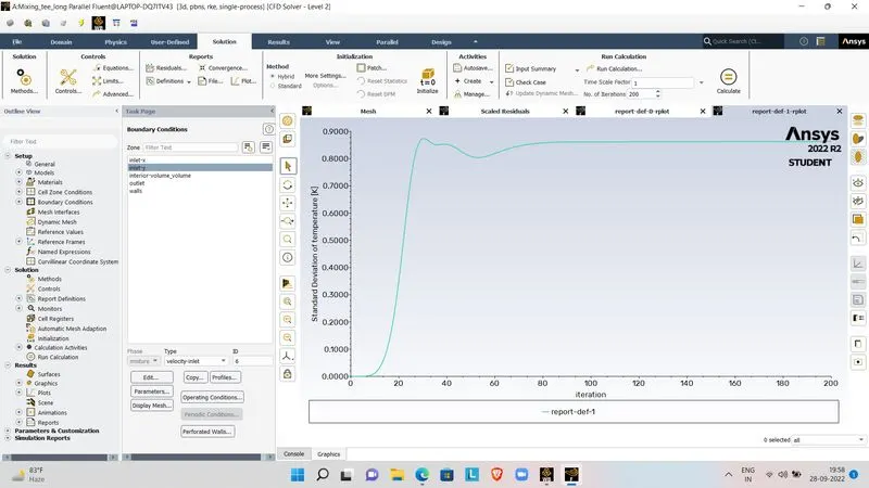
STANDARD DEVIATION:

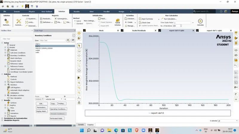
AREA WEIGHTED AVERAGE TEMPERATURE:

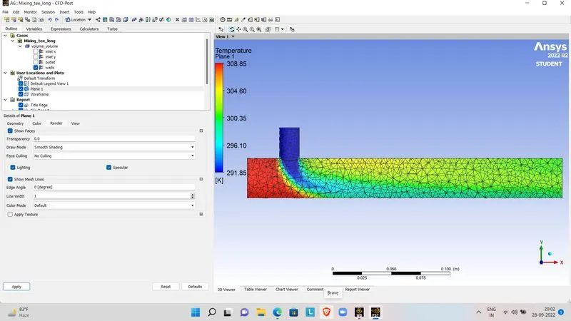
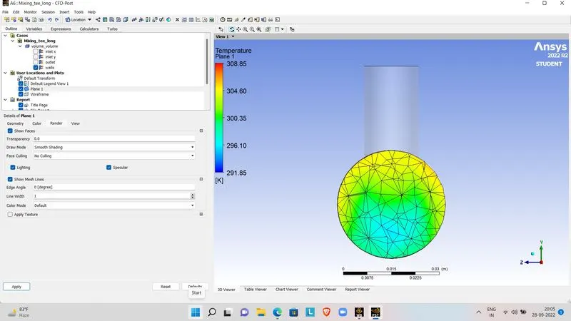
CONTOUR PLOTS:

TEMPERATURE PLOTS:

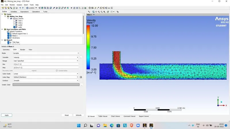
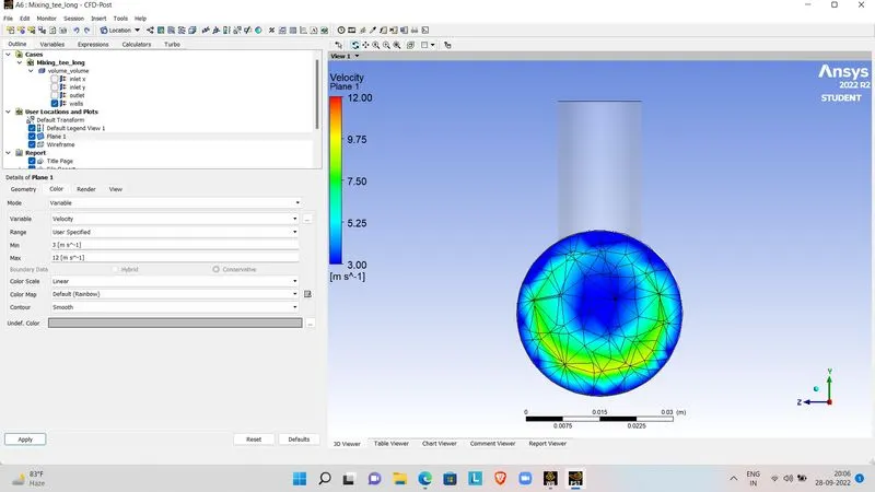
VELOCITY PLOT:

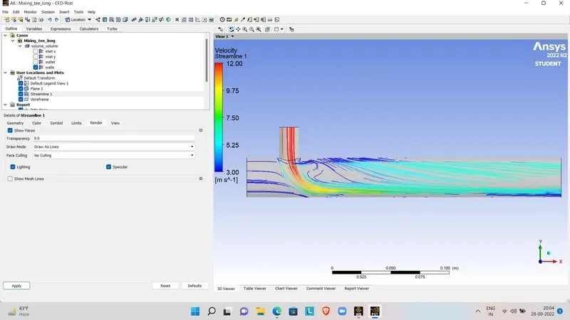
STREAMLINE PLOTS;

VELOCITY PLOT:

TEMPERATURE PLOT:

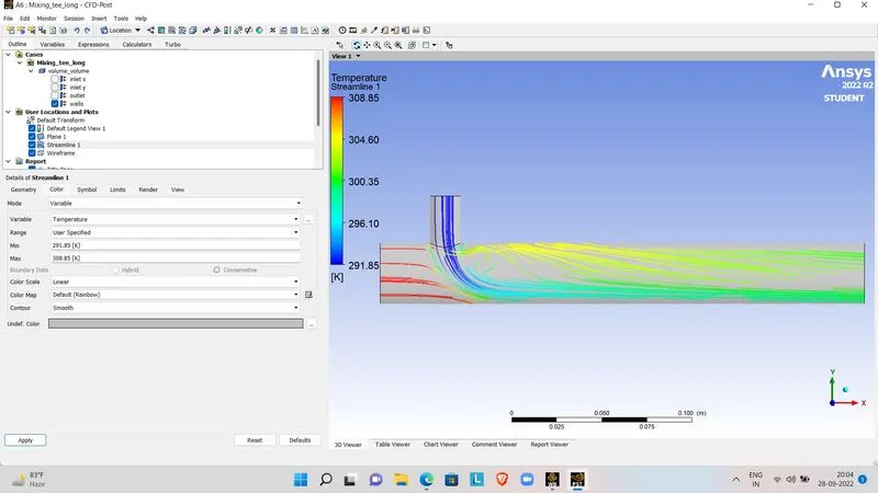
SUMMARY FROM ABOVE OBSERVATIONS:

	LONG TEE (MR = 2)	LONG TEE (MR = 4)
AVERAGE OUTLET TEMPERATURE [K]	303.39	300.34
STANDARD DEVIATION	1.2	0.8
NO OF ITERATIONS	160	130

COMPARISON OF BOTH LONG AND SHORT TEE:

K-EPSILON REALIZABLE MODEL
GEOMETRY	MOMENTUM RATIO	CELL COUNT	AVERAGE OUTLET TEMPERATURE [K]	NO. OF ITERATIONS	STANDARD DEVIATION
SHORT TEE	2	12608	303.32	150	1.5
SHORT TEE	4	12608	300.34	140	1.1
LONG TEE	2	15549	303.39	160	1.2
LONG TEE	4	15549	300.34	130	0.8

OVERALL CONCLUSION:

• Irrespective of the length of the mixing Tee, the average outlet temperature in both cases is quite the same. But longer mixing tee is preferred for better mixing of fluids and better outlet temperature.
• As the momentum ratio increases, the velocity of cold inlet fluid increases, and due to the high relative velocity between the fluid it experiences higher turbulence, and therefore the outlet fluid temperature decreases.
• Momentum Ratio is inversely proportional to the outlet temperature.
• In order to obtain better mixing the velocity of cold air is important. By increasing the cold fluid velocity the outlet temperature gets reduced.
• The longer Tee takes more time to converge than the short Tee.
• Therefore, it is efficient to use the short mixing tee with MR=4.

GRID INDEPENDENCY TEST:

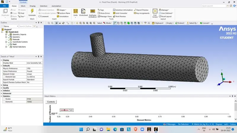
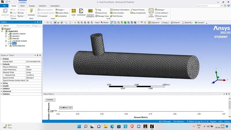
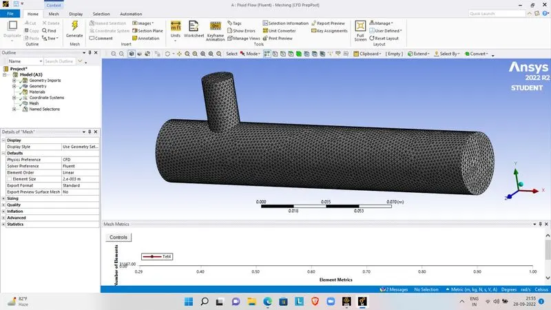
Short Tee model is selected for grid dependence test.

MESH GENERATION:

5mm:

3mm:

2mm:

CONCLUSION:

SUMMARY:

MESH SIZE	NO. OF ELEMENTS	NO. OF NODES	AVERAGE OUTLET TEMPERATURE	NO. OF ITERATIONS
5mm	14302	3154	30.09	60
3mm	40,031	8385	30.12	70
2mm	106236	21390	30.13	75

CONCLUSION:

• From the above table we can say that our mesh is independent which means there are no large changes in outlet temperature by increasing the number of elements.
• Decreasing the mesh size, the average outlet temperature starts approaching the analytical results.
• The main advantage of this study is to decrease the computational time for solving.
• As the mesh size decreases, standard deviation increases because as the number of cells increases, the temperature is calculated more accurately increasing deviation in calculated values from one cell to another cell.