Week 1- Mixing Tee

Week 1- Mixing Tee

Aim:

To perform CFD Flow analysis on the given Short mixing Tee and Long mixing Tee models for the mixing effectiveness of hot and cold fluids mixing at the Tee interface for two momentum ratios. Interpret the results of the mixing and conclude the case comparison.

Introduction:

The given models are Short mixing Tee and Long mixing Tee models in which two moving fluids at different temperatures mix. This is a common everyday case scenario in home and industrial applications, here we are going to study the physics of the mixing and come up with solutions that enhance the mixing. We are given some input datas to start our simulation,

As per the given data, we have

1. Case 1
• Short mixing tee with a hot inlet velocity of 3m/s. Thot =36 C & Tcold=19 C
• Momentum ratio of 2.( Vhot = 3 m/s, VCold = 6 m/s)
2. Case 2
• Short mixing tee with a hot inlet velocity of 3m/s. Thot =36 C & Tcold=19 C
• Momentum ratio of 4.( Vhot = 3 m/s, VCold = 12 m/s)
3. Case 3
• Long mixing tee with a hot inlet velocity of 3m/s. Thot =36 C & Tcold=19 C
• Momentum ratio of 2.( Vhot = 3 m/s, VCold = 6 m/s) .
4. Case 4
• Long mixing tee with a hot inlet velocity of 3m/s. Thot =36 C & Tcold=19 C
• Momentum ratio of 4.( Vhot = 3 m/s, VCold = 12 m/s) .

Theory of the topic and its importance in practical applications:

A tee is formed by two pipe sections joined at a right angle to each other. One stream passes straight through the tee, while the other enters perpendicularly. This flow arrangement is known as the Side Tee. There are other Tee models such as opposed Tee mixer and Multiple Tee mixer that find a wide variety of applications in industries in which two fluid streams with different physical and/or chemical properties mix—are widely used in the petrochemical industry.

When there is a large temperature difference between two streams, large metal temperature fluctuations can occur in the region where the two streams meet if proper design steps are not taken. The temperature fluctuations in the metal can lead to thermal fatigue of the pressure boundary piping. If through-wall cracking occurs, the fluid may leak, possibly causing a fire and damage. Therefore, it is imperative to ensure that the piping system can withstand the temperature fluctuations.

This type of mixing Tees are found in petroleum industries, Thermal power plants, HVAC applications, Centralized air condition systems, Nuclear power reactors. Basically, wherever two fluid streams with different velocity and temperatures mix. So, study of this mixing is very much important to design these fluid flow systems.

Solving and Modeling approach:

Mixing Tee model effectiveness can be studied by analytical approach, experimental approach and simulation approach. Ideally, an analytical approach gives us exact results but it is time consuming and not much flexible in terms of practicality. Experimental approach is costlier. In this situation, simulation comes handy, flexible, time saving.

We will be using ANSYS Fluent solver to import the geometry and extract fluid volume, perform unstructured tetra CFD mesh with boundary definitions, setup the physics of fluid flow and run the iterations to get solutions, using post processing to interpret the data in form of plots,contours, vectors etc.,

Then, we tabulate the case study results and compare it with the analytical results to validate the simulation.

Preprocessing and Solver setting:

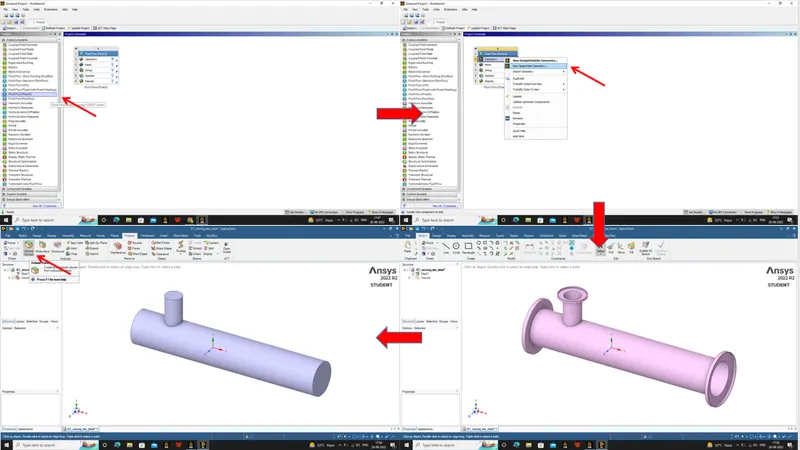
Let us open ANSYS workbench, now opening Fluent flow can be done by drag and drop in the schematic window or by double clicking on Fluent. The fluent workflow is in a series of steps such as GEOMETRY > MESH > SETUP > SOLUTION > RESULTS. Each step has to be completed for the next step to initialize.

Let us discuss case 1 in detail;

GEOMETRY >

In the Fluent, right click on the Geometry and select New SpaceClaim Geometry. The spaceclaim application opens, select FILE > OPEN and open the short mixing Tee model from the model explorer.

As our area of interest is the fluid volume, we will extract the fluid volume using the VOLUME EXTRACT option and selecting the edges of the openings. We can suppress the shell element for physics by right clicking the shell.

Once the geometry is ready, we can close spaceclaim and check that the fluid flow (fluent) geometry is updated indicated by a green tick.

MESH >

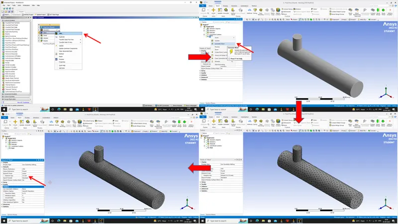
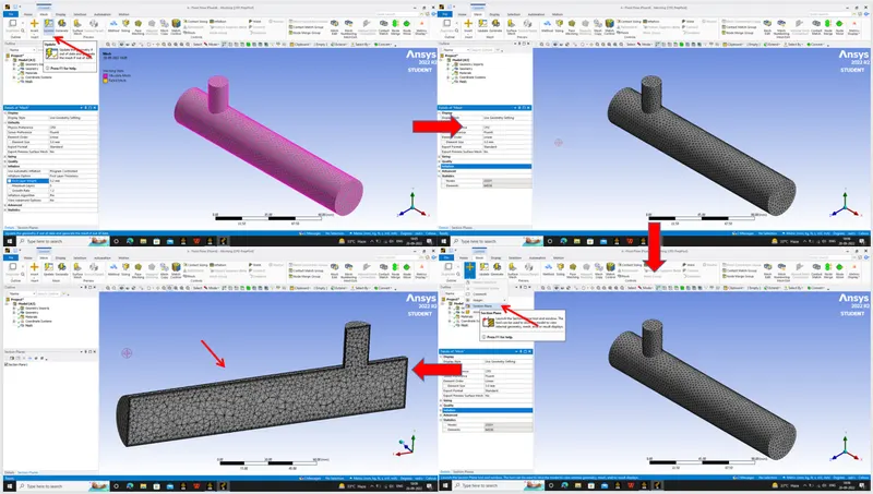
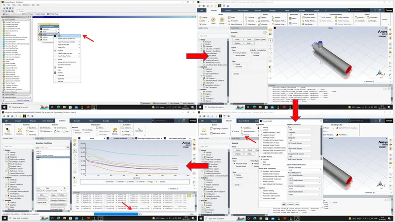
Right clicking on the Mesh and selecting edit opens the Mesh window. Mesh window is preloaded with the geometry we have worked on earlier, so clicking on the GENERATE MESH should create a mesh automatically. Our interest is target element length of 3 mm, to change that click on the mesh and edit in the details tab. We can even add inflation layers there and check the same by creating a section plane. Any changes made, click on the update icon to update the mesh details or else there is an indication of a thunderbolt sign asking the user to update.

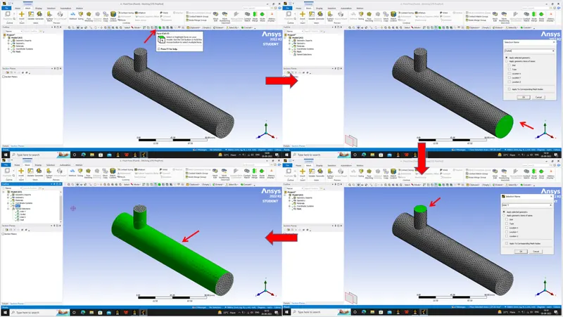
We shall name the entry and exit surfaces such as Inlet X, Inlet Y, Outlet, Wall by selecting the respective faces and using the ‘N’ button. Once this is done, we should see a green tick near Mesh. we can close the mesh window.

SETUP >

Right clicking on the Setup, opens the Fluent launcher. In the Fluent launcher select 3D, Double precision and select the number of cores as per the user system configuration and click on start.

Upon opening, there are some selections to be done to define the simulation definitions, we shall select Type: Pressure based, Velocity Formulation: Absolute, Time: Steady. Under the Physics tab, we can turn on energy and select k-epsilon (2 eqn) in the viscous.

Under the materials we shall select air as our default material with material type as fluid.

Under the cell zone conditions, select the volume and it should show type as fluid by default.

We can proceed to define boundary conditions, as follows

Inlet X : velocity magnitude = 3 m/s and temperature = 36 C,

Inlet Y : velocity magnitude = 6 m/s and temperature = 19 C,

Outlet should be a pressure outlet.

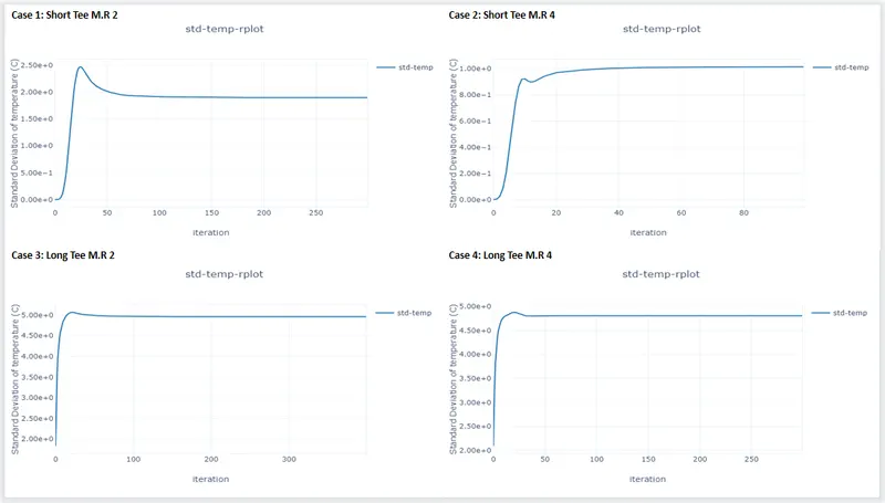
For generating surface reports, click on the Solution > Reports > Definitions > New > Surface Report > Area-Weighted Average for the average temperature across the outlet. And instead of selecting Area-weighted average and selecting Standard deviation gives the standard deviation of outlet temperature.

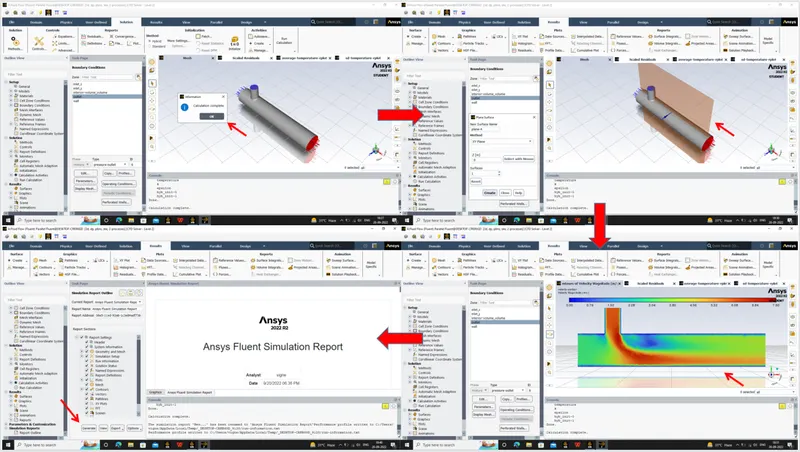
Now, it's time to start the simulation. In order to start the simulation for the above set up physics, we need to initialize the entire flow field by clicking on the t=0 initialize icon. In the Run Calculation we can input the number of iterations to be run (in this case 300) and clicking on the Calculate should start the iterations. After iterations, we get scaled residuals, average temperature plot and standard deviation plots.

We need velocity and temperature contours as well, to get them we can create a transverse cut plane i.e, XY plane and make new contour in Results > Graphics > Contours > New select the cut plane and temperature for temperature contour and velocity for velocity contour. The scale can be edited by double clicking on it.

In the Outline view under Simulation Reports, clicking on the Report Outline > Generate should generate a Ansys Fluent Simulation Report which is automatically generated with all the information of the simulation in it. This can be exported as a PDF also. We are done with setup, we can close the setup.

SOLUTION >

Since some solution is calculated in the setup itself, we can see the green ticks in both setup and solution too.

RESULTS >

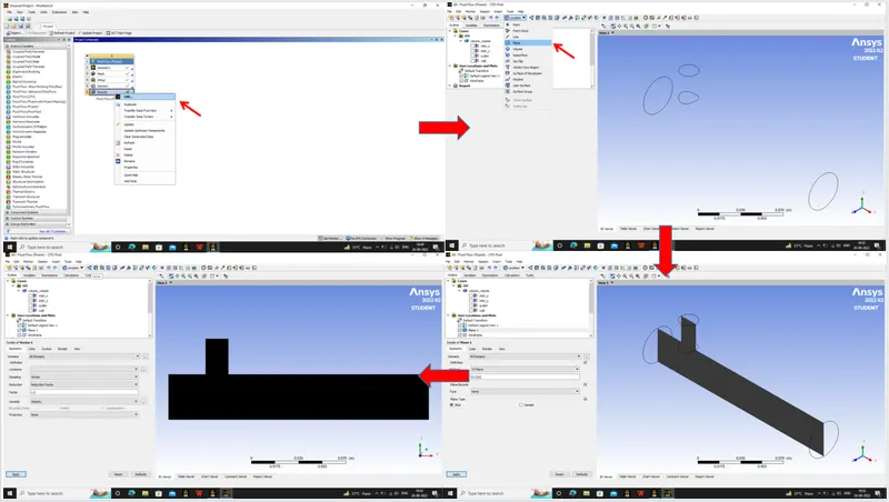
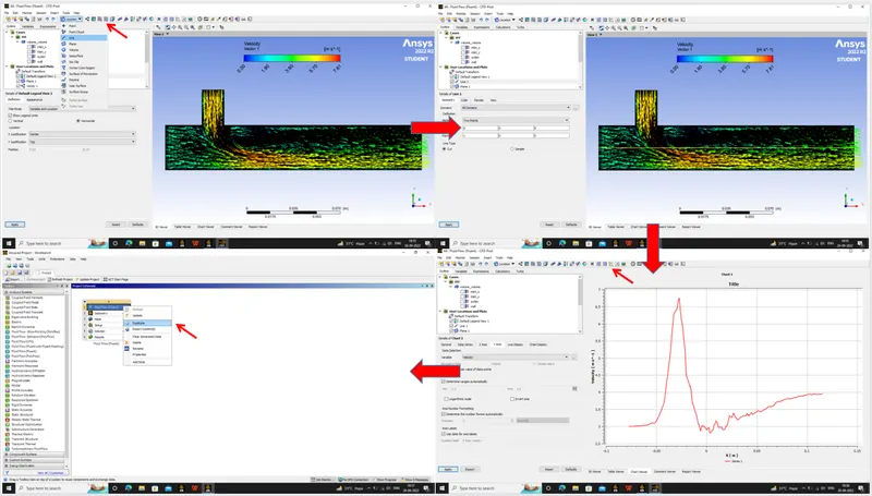
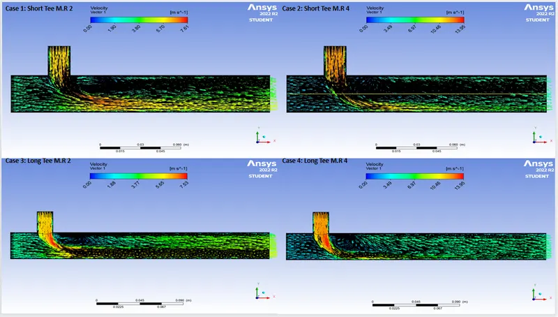
Right clicking on the Results should open the Post processor. Default view is a wireframe model, we can create a transverse section plane by Location > Plane and color it black. Selecting the Vector and selecting the section plane creates a velocity vector.

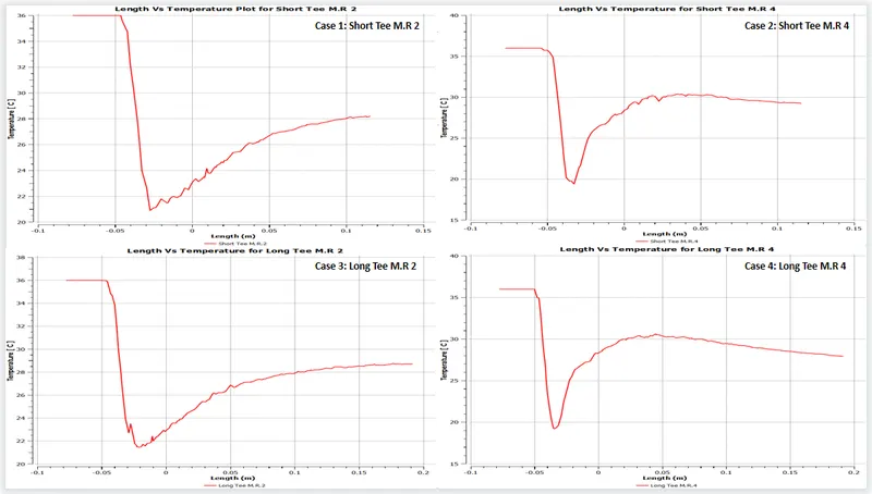
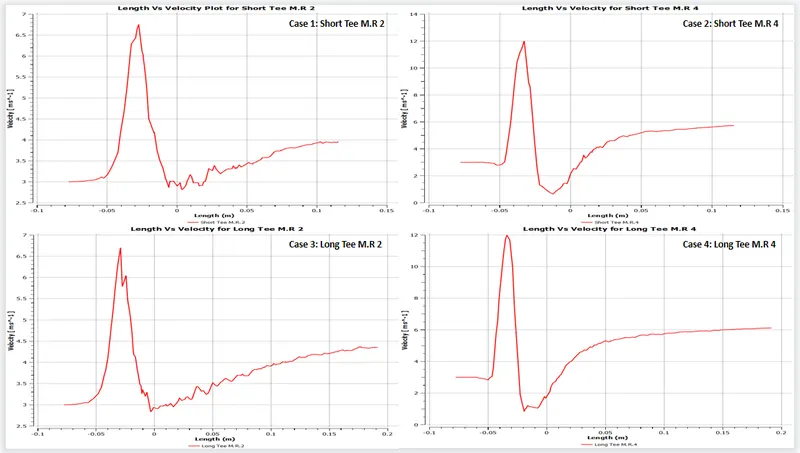
Similar to plane creation, we can create a Line that cuts through the central axis. This line can be used to collect data and plot temperature and velocity across the length of the model using the Plot option. Several options can be changed as per user requirement in the plot option.

We can use the Probe tool to find required parameter like pressure, velocity, temperature at any point in the cut section plane.

For Case 2, we can simply Duplicate the existing Case 1 Fluent file. Change the Inlet Y velocity in the Setup and run the simulation and gather data like we did with case 1.

Similarly, we can follow the above procedure for the Long Mixing Tee model as well for Case 3 and Case 4.

RESULTS:

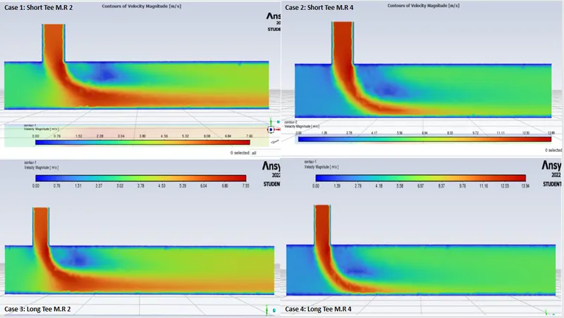
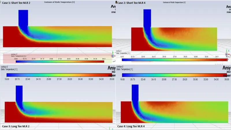
After repeating the similar manner of simulation procedures for all other 3 cases, we have a handful of datas to compare and study. We shall put in order all the contours, plots and vectors for us to compare all 4 cases and come to a conclusion. Here, only the results of all cases are displayed, its inference and interpretation shall be discussed briefly in conclusion.

Contour of Velocity Magnitude [m/s]

Contour of Temperature [C]

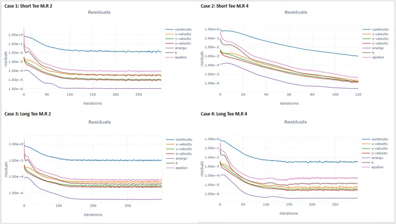
Residuals

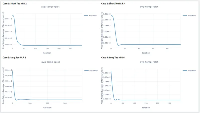
Average Temperature

Standard Deviation

Velocity Vectors

Length Vs Temperature Plot (at core)

Length Vs Velocity Plot (at core)

CONCLUSION:

From the results we obtained from all 4 cases and its comparison visually from the graphs and contours we can say that case 2 is better among the 4. Let us see the analysis data from the simulation as well in the below tabulation for mesh element size 3mm and k epsilon model.

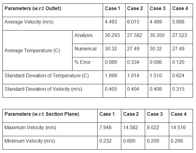
INFERENCES:

The average temperature in C at the outlet is almost similar to the numerical values, whereas momentum ratio 4 seems to have good mixing and in case 2 and case 4 comparison, length doesn’t seem to affect the outlet temperature. Velocity of the cold fluid is having a significant role in mixing effectiveness and the outlet temperature. The same can be inferred from the standard deviation values of both temperature and velocity.

The average velocity seems to decrease with increase in length in comparison from case 2 and case 4 average velocities.

At the cut section plane, the velocity is maximum at the interface of the mixing zone and a vortex is created as a negative pressure region due to the 90 degree angle of the Tee joint (The same can be observed in velocity contours and velocity vectors). In order to avoid this negative pressure region, we can make angular Tee or introduce some radius or chamfer at the internal region of the Tee intersection.

So, in my observation case 2 is better among the 4 cases in terms of convergence as well. Case 2 converged at 127 iterations while other cases only continuity seemed to not converge even at over 300 iterations. To improve the case 2 model, modifying the case 2 with angular Tee at say 45 or 60 degrees entry angle may improve the mixing efficiency while removing the negative pressure zone as well.

Hence, the Week 1 challenge is completed with the snippets attached wherever required.

References:

1. https://www.sciencedirect.com/science/article/pii/S0029549309005676

2.https://www.researchgate.net/publication/332494613_COMPARISON_OF_CFD_SIMULATION_OF_HOT_AND_COLD_FLUID_MIXING_IN_T-PIPE_BY_PLACING_NOZZLE_AT_DIFFERENT_PLACES