Week 1- Mixing Tee

Aim: To set up steady-state simulations to compare the mixing effectiveness when hot inlet temperature is 36⁰C & the Cold inlet is at 19⁰C creating two version of mixing tee

Objective:

• to set up steady-state simulations to compare the mixing effectiveness when hot inlet temperature is 36⁰C & the Cold inlet is at 19⁰C.
• Use the k-epsilon and k-omega SST model for the first case and based on your judgment use the more suitable model for further cases. Giving the reason for choosing a suitable model is compulsory.

1. Case 1
   • Short mixing tee with a hot inlet velocity of 3m/s.
   • Momentum ratio of 2, 4.
2. Case 2
   • Long mixing tee with a hot inlet velocity of 3m/s.
   • Momentum ratio of 2, 4.

Momentum ratio = velocity at cold inlet / velocity at hot inlet

In a table, compare the following values from the 2 cases.

1. Cell count
2. Average outlet temperature
3. Number of iterations for convergence

Expected results:

1. Velocity and temperature contour plots on the cut planes along and across the pipe.
2. Velocity and temperature line plots along and across the length of the pipe.
3. Perform Mesh independent study for any one case.
4. Discuss the effect of length and momentum ratio on results

Procedure:

• We will start with first case of short mixing tee with hot inlet velocity of 3m/s and momentum ratio of 2 i.e., velocity at cold inlet will be 6m/s. We will use both K-epsilon and K-omega SST method to converge the solution and choose the best between the two and same would we used for other cases.We Initiate the project by dragging and dropping the Fluid Flow(fluent) into the project schematic window.
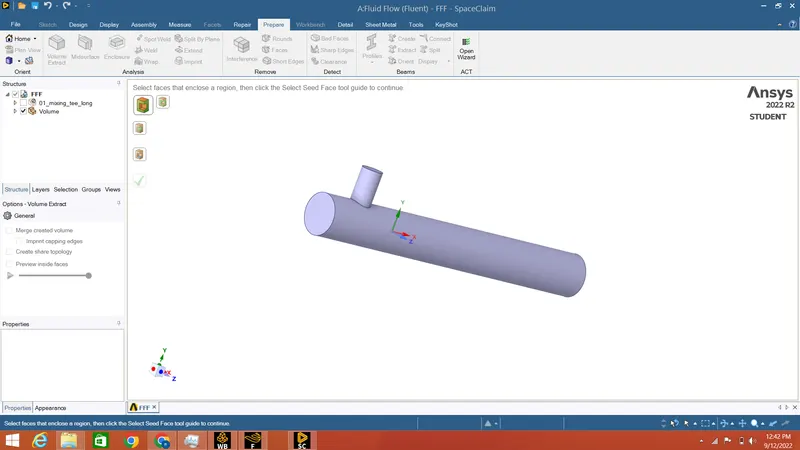
• After that Geometry model was setup using space-claim where we opened our 3D cad file of model and after that extracted the fluid volume with “volume extract” method in which we used the edge selectin tool to select the boundary edges of thee fluid flow volume.
• Once this was done we suppressed the outer geometry or shell by using the suppress for physics option in order to keep it away from interfering with the simulation.

• After that we closed the Space-claim and Initiated mesh, where we used Face selection tool to select the boundaries of the fluid flow volume and we named the boundaries accordingly.

• Next we right clicked on the mesh option from left tool bar and generated mesh. In the available options to see mesh details we plotted the mesh quality graph.

• 
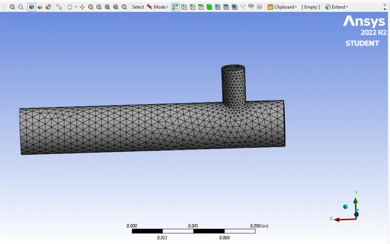
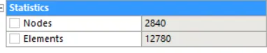
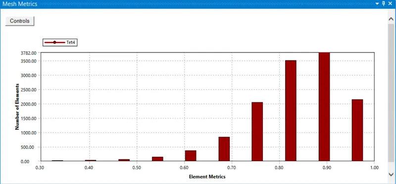
• Once the mesh was done, we initiated Setup which uses Ansys fluent, in the launcher we selected 4 processors coz that was max allowed by our license. After that In fluent the first thing we performed was mesh check, after we got ok from there we went into physics where we setup the general settings like units and things and in the zones we gave all our simulations Initial conditions after which we selected Energy equation and in viscous we selected the model type of our choice. After that we used the definition tool to specify the plot outputs we wanted from the simulation and then we initialised the solution it ran for 10 iterations and once it was done we calculated values for 150 iterations and then closed the Ansys fluent.
• after the put all parameters we initiallized the project and calculate with the 150 iterations
• k-omega short tee with the moment ratio of 2
• Case 1
  • Short mixing tee with a hot inlet velocity of 3m/s.
  • Momentum ratio of 2, 4.
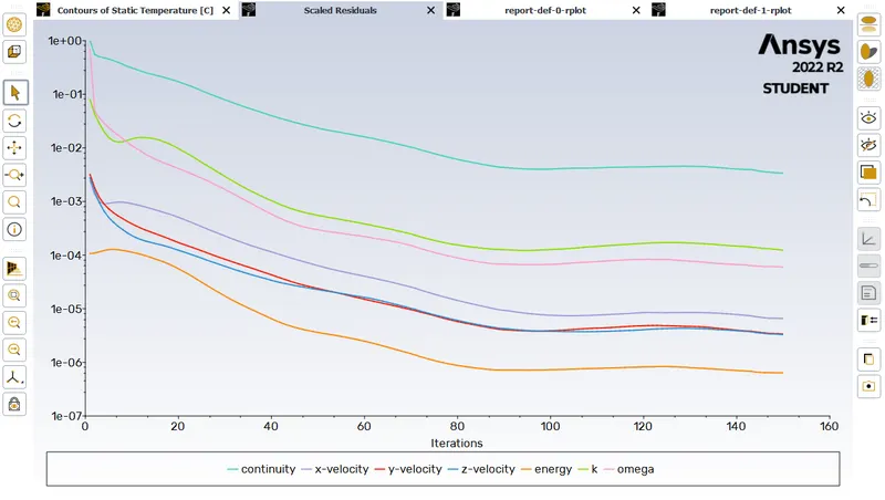
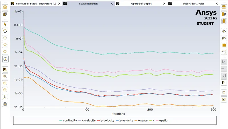
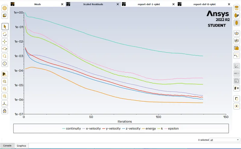
• scaled Residual of k-omega with the Momentum ratio of 2
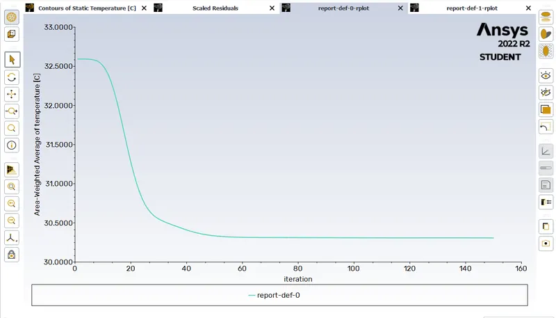
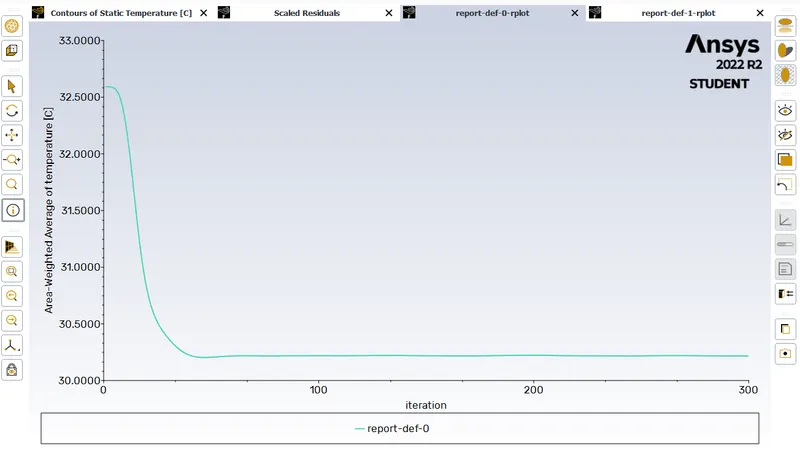
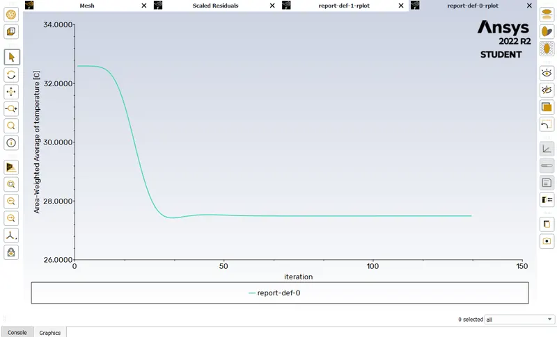
• Area-weighted at temperature with the Momentum ratio of 2
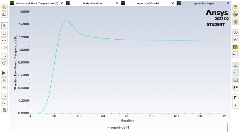
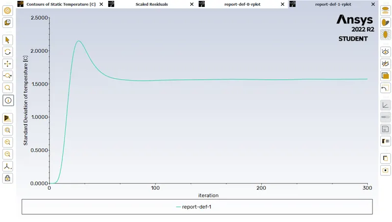
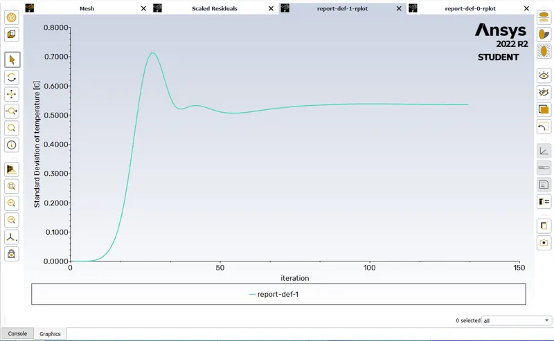
• Standard Deviation at k- omega with the Momentum ratio of 2
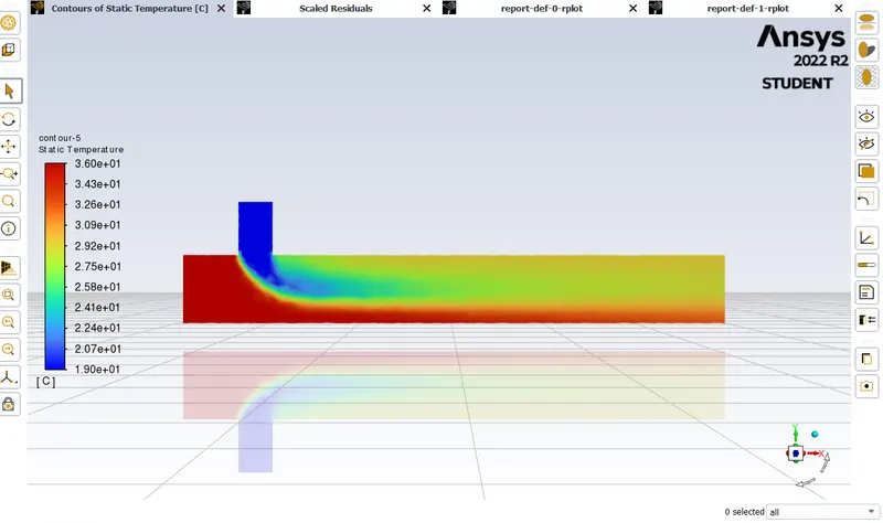
• temperature contour at k-omega at with the Momentum ratio of 2
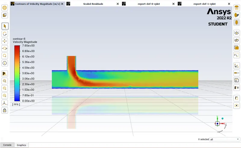
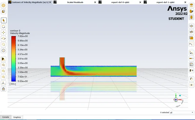
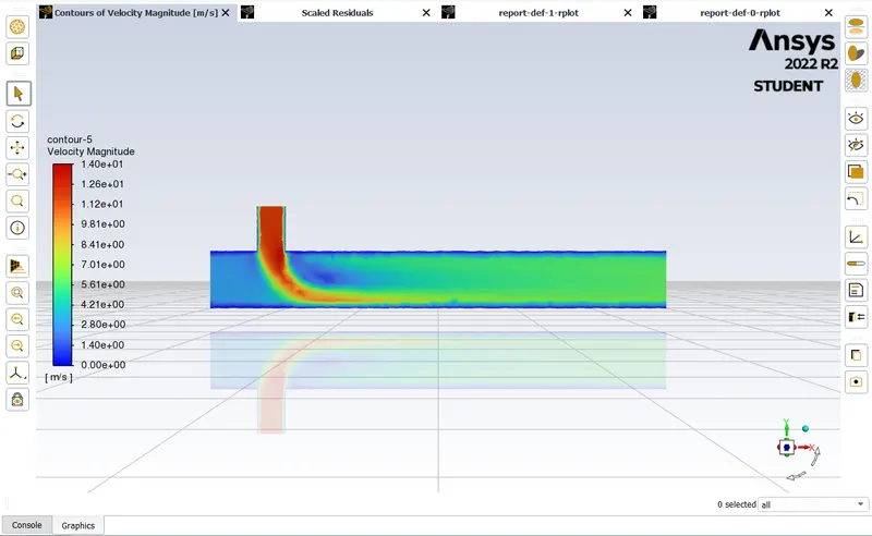
• Velocity contour at k-omega at with the Momentum ratio of 2

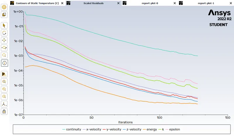
• scaled Residual of k-epsilon with the Momentum ratio of 2
• Area weighted at the temperature of k-epsilon with the Momentum ratio of 2
• Standard deviation of k-epsilon with the Momentum ratio of 2
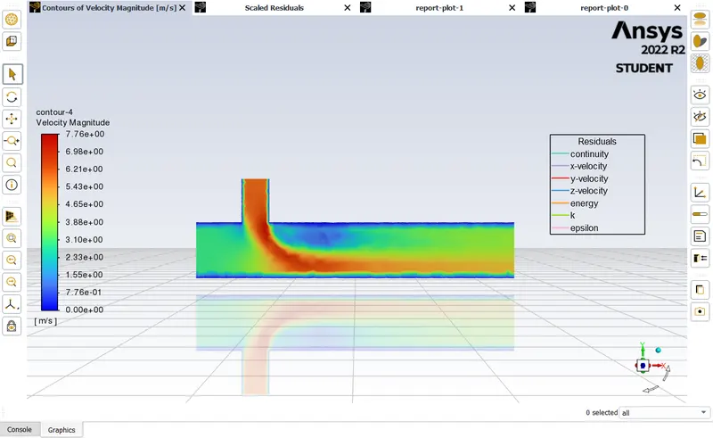
• Temperature contour of k-epsilon with the Momentum ratio of 2
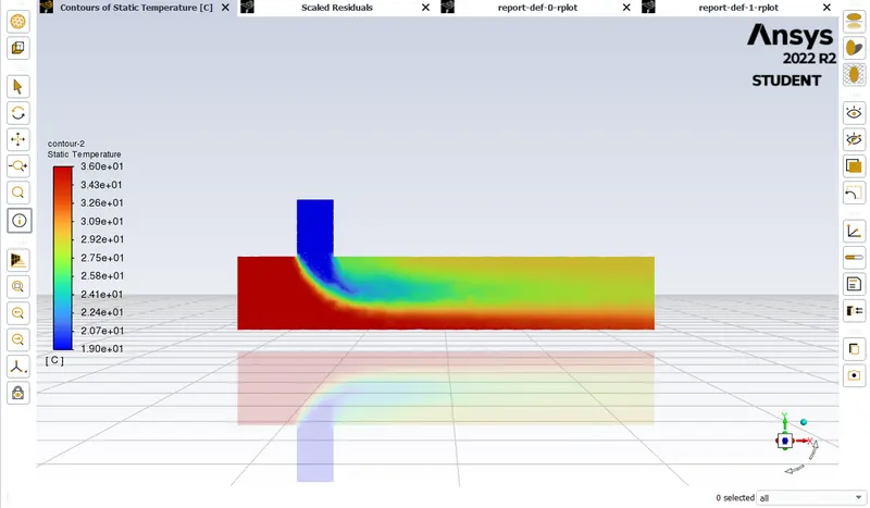
• velocity contour of k-epsilon with the Momentum ratio of 2
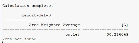
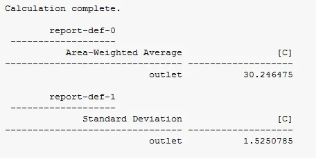
• Temperature at outlet
• 
• scaled Residual of k-epsilon with the Momentum ratio of 4
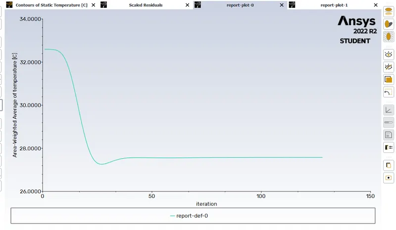
• Area weighted at temperature of k-epsilon with the Momentum ratio of 4
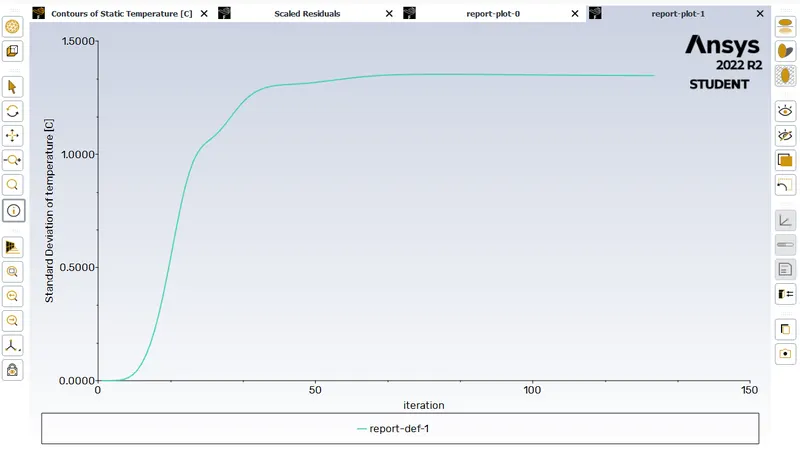
• Standard Deviation of k-epsilon with the Momentum ratio of 4
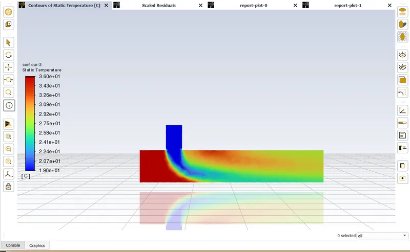
• Temperature Contour of k-epsilon with the Momentum ratio of 4
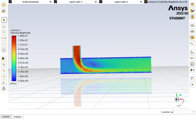
• Velocity Contour of k-epsilon with the Momentum ratio of 4

• Case 2 Long Mixing Tee
  • Long mixing tee with a hot inlet velocity of 3m/s.
  • Momentum ratio of 2, 4.

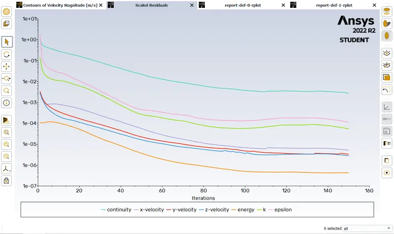
• Scaled Residual with the Momentum ratio of 2

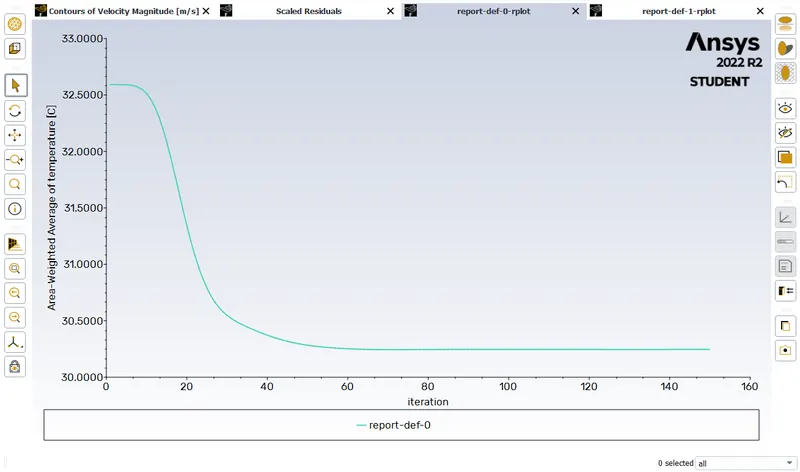
• Area weighted at temperature with the Momentum ratio of 2

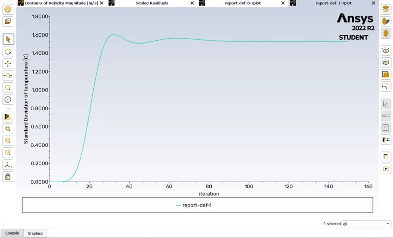
• Standard Deviation with the Momentum ratio of 2

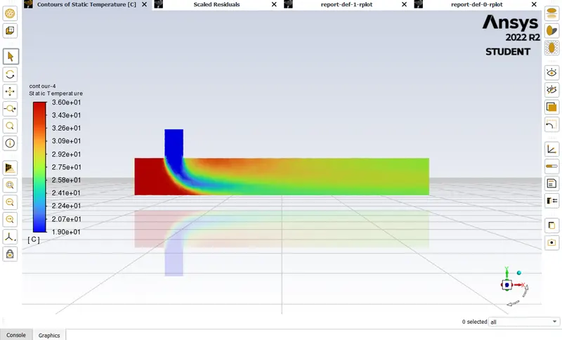
• Temperature Contour with the Momentum ratio of 2

• Velocity Contour with the Momentum ratio of 2

• Scaled Residual with the Momentum ratio of 4

• Area weighted at temperature with the Momentum ratio of 4

• Standard Deviation with the Momentum ratio of 4

• Temperature Contour with the Momentum ratio of 4

• Velocity Contour with the Momentum ratio of 4

Temperature at outlet

Conclusion:

As seen in the Case-1and Case-2, the temperature at the outlet drops down significantly due to high velocity of cold air from the inlet. This is possible due to the turbulent mixing at the tee joint between hot air and cold air because of the high velocity of cold air., which is not possible in case of low-velocity cold air.

The temperature contour at the outlet for short tee cases shows that some of the high temperatures flow sips through without properly mixing with the flow. Whereas, in the temperature contour of long tee cases, the high temperatures flow thoroughly mixes with the rest of the flow.
Therefore, we can recommend using the long tee and high-velocity inlet for application. This is because we have a low standard deviation in case of long tee compared to the short tee for both momentum ratios.

k- epsilon model predicts well far from the boundaries (wall) and k- omega model predicts well near the wall. Even though it depends on Y+. Therefore, K-epsilon model is majorly used for free flow away from the wall and as in this project, there is no dealing with the wall of the mixing tee for change in temperature along the length of it, so K-epsilon model was chosen for further simulations.