1. Introduction

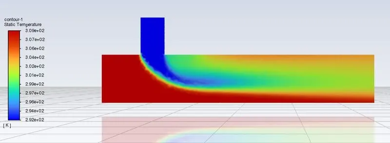
The objective of the project is to perform steady state simulation to determine the mixing effectiveness when hot air with temperature 36°C mixes with the cold air with temperature 19°C in mixing tee joint

2. Problem Statement

For this challenge, we have created two versions of the mixing tee. One of them is longer than the other.

Your job is to set up steady-state simulations to compare the mixing effectiveness when hot inlet temperature is 36⁰C & the Cold inlet is at 19⁰C.

Use the k-epsilon and k-omega SST model for the first case and based on your judgment use the more suitable model for further cases. Giving the reason for choosing a suitable model is compulsory.

1. Case 1
   • Short mixing tee with a hot inlet velocity of 3m/s.
   • Momentum ratio of 2, 4.
2. Case 2
   • Long mixing tee with a hot inlet velocity of 3m/s.
   • Momentum ratio of 2, 4.

3. Problem Setup for Simulation

3.1 Geometry Setup

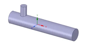
1. The geometry provided is imported into SpaceClaim for extracting the volume of the geometry as the main aim of the assignment is to understand the flow within this volume.
   
   
   
   
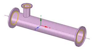
2. The Volume is created in the component on which simulation is needed to be performed. The remaining solid structure is to be suppressed as it is not necessary for the simulation.
   
   

3.2 Mesh Setup

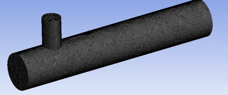
1. A Mesh is being used to obtain a mesh of Triangles considering an element size of 0.0040 m.
   
   
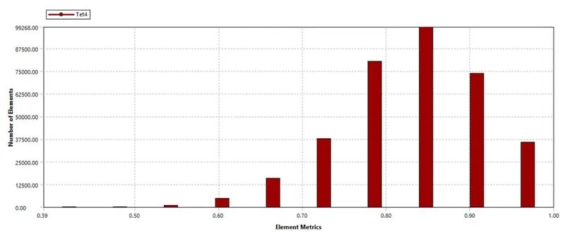
2. The Mesh Quality is obtained above 5%.
   
   
   
   
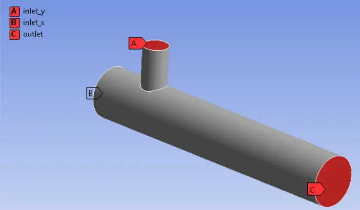
3. The named sections are given as below

3.3 Solver Setup

1. For Steady State simulation, Steady is selected in the Time Section of the General Tab.
   
   
   
   
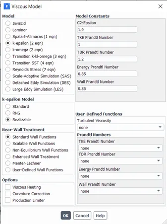
2. For all the scenarios, k-epsilon or k-omega is to be selected based on the evaluation with realizable Standard Wall Function and SST for k-omega.
   
   
   
   
3. The material properties are to be setup as per the Parameters mentioned in the above section for all the cases.
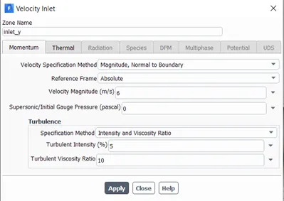
4. The inlet velocity is to be calculated based on the given below Formulae.
   
   
   
   
   
   
   
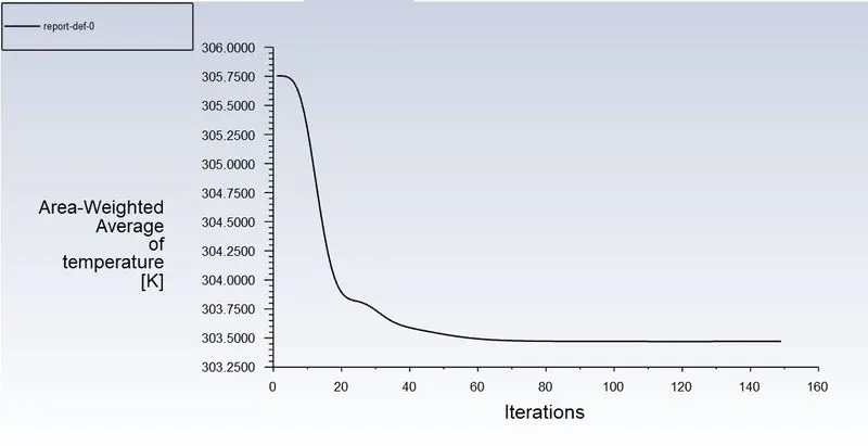
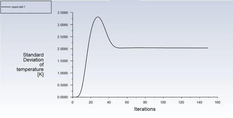
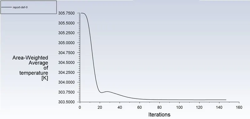
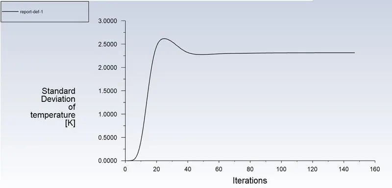
5. two reports to extract information about the temperature distribution on the outlet face of the mixing tee, the Area weighted average of temperature & standard deviation reports has been setup from the definition tab available in Solution > Report tab
6. The Setup is Initialised, and the number of iterations is set to 1000 Iterations to obtain the required result.

4. Simulation Results

4.1 Case - 1 (MR = 2, k-epsilon Realizable with SWT)

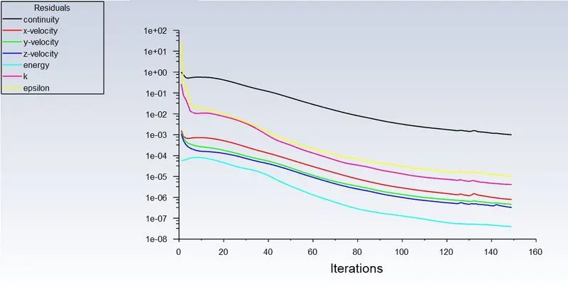
1. Residual Scaled Graph
   
   
   
   
2. Area Weighted Average Temperature
   
   
   
   
3. Standard Deviation of Temperature
   
   
   
   
   
4. Temperature Contour
   
   
   
   
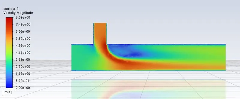
5. Velocity Contour
   
   

4.2 Case - 1 (MR = 2, k-omega SST)

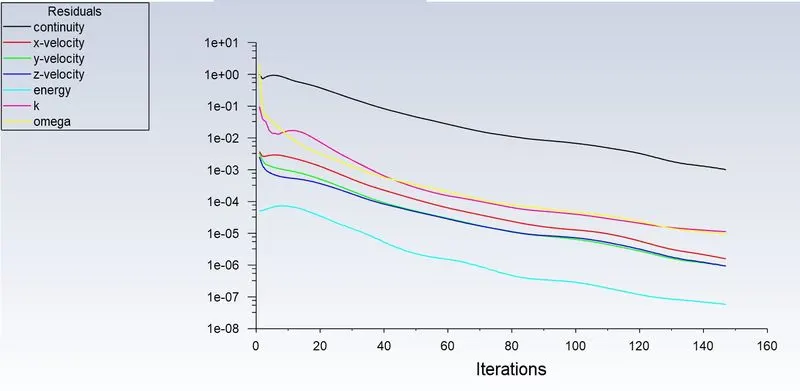
1. Residual Scaled Graph
   
   
   
   
2. Area Weighted Average Temperature
   
   
   
   
3. Standard Deviation of Temperature
   
   

4.3 Case - 1 (MR = 4, k-epsilon Realizable with SWT)

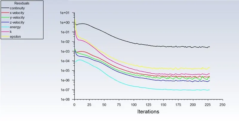
1. Residual Scaled Graph
   
   
   
   
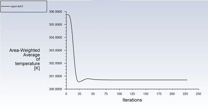
2. Area Weighted Average Temperature
   
   
   
   
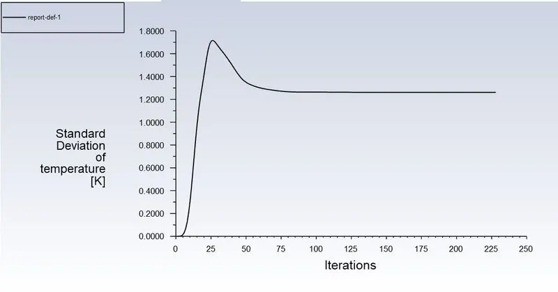
3. Standard Deviation of Temperature
   
   
   
   
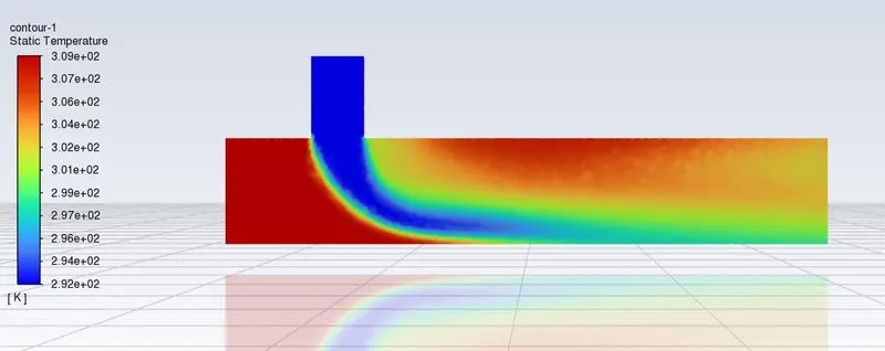
4. Temperature Contour
   
   
   
   
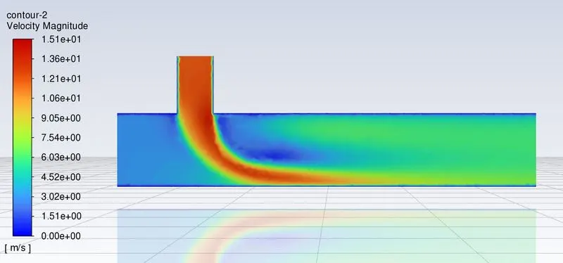
5. Velocity Contour
   
   

4.4 Case - 1 (MR = 4, k-omega SST)

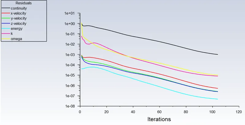
1. Residual Scaled Graph
   
   
   
   
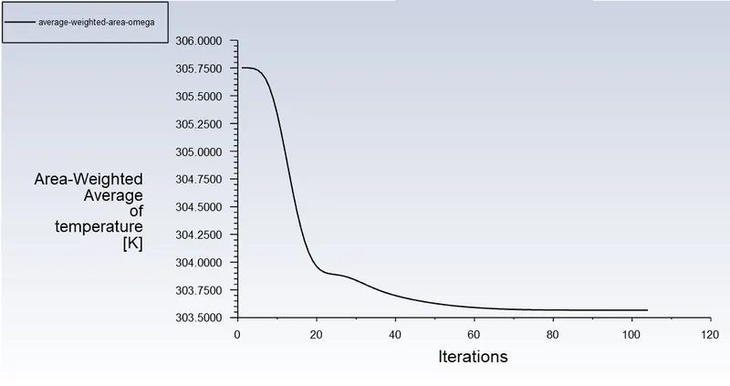
2. Area Weighted Average Temperature
   
   
   
   
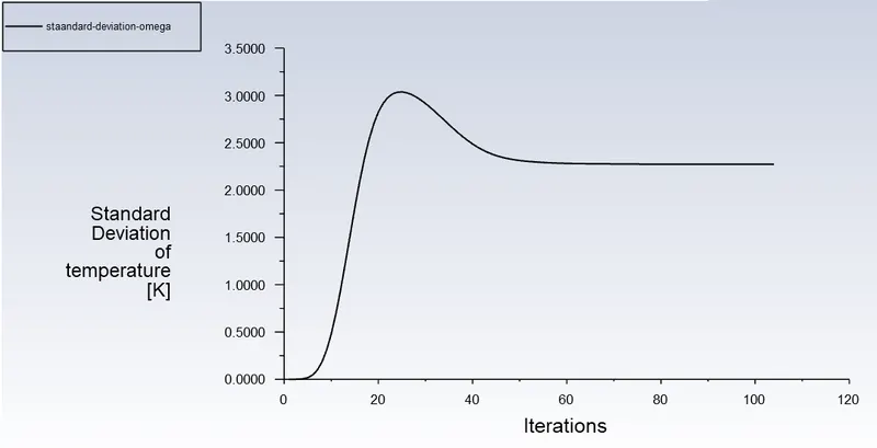
3. Standard Deviation of Temperature
   
   
   
   
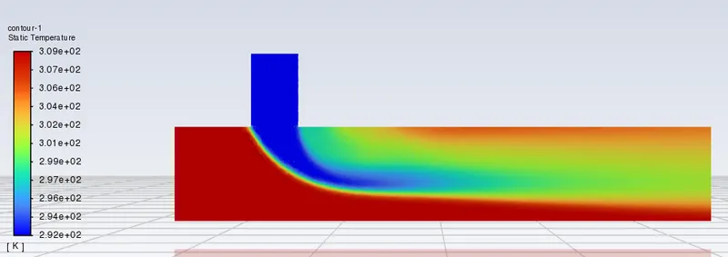
4. Temperature Contour
   
   

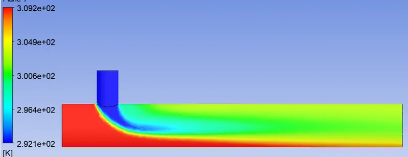
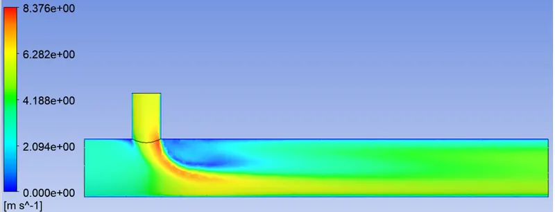
4.5 Case - 2 (MR = 2, k-omega SST)

1. Temperature Contour
   
   
   
   
2. Velocity Contour
   
   

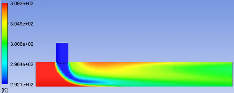
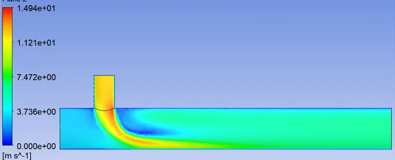
4.2 Case - 2 (MR = 4, k-omega SST)

1. Temperature Contour
   
   
   
   
2. Velocity Contour
   
   

5. Discussion of Results and Conclusion

3.3 Difference between k-epsilon and k-omega functions

k-epsilon

the fundamental transport-equation model that accounts for turbulent dispersion and kinetic energy. The rate where the velocity irregularities diminish is known as turbulent dispersion. That's the K-model by default. Equations are obtained experimentally and are applicable to highly turbulence models. The Reynolds stresses are related to the mean velocity gradients and the turbulent viscosity using the gradient diffusion hypothesis in the k-e model. underperforms for complex models with a significant profile curves, divergence, and differential pressure. One of most alarming flaw is the lack of consideration to negative pressure distribution; additional flaw is computational rigidity when solutions are averaged through fluid domain and handled with unstable dampening coefficients.

k-omega

It is a method with transport equations that solves for turbulence frequencies and kinetic energy. That's the K-model by definition. With an instantaneous move from a wall function to a low-Reynolds number composition depending on separation distance, this framework encourages a much more precise near wall handling. increased performance for low Reynolds number and wall-bounded streams. demonstrates possibilities for transitional prediction.

The conventional k-model has a variation called shear stress transport (SST). uses a mixing mechanism to integrate the conventional k- model far from walls and the classic Wilcox k-w model for use near walls. The eddy viscosity equation is also changed to compensate again for impacts of primary turbulent shear stress on transport.

The SST variation of the k-omega model benefits from both the k-epsilon and conventional k-omega models. Because of this, the k-omega SST model will be employed for the remaining cases.

The results from the mesh independent study are as tabulated below

Mesh Independent Study
Geometry	Element Size (mm)	Cell Count	Averge Outlet Temperature (°C)
MR - 4	0.1	450668	27.1402
	0.5	420523	27.623
	1	385632	27.953

Based on the above simulations, the tabular data represents the overall summary of the simulation for all the cases.

Case	Case Type	No. of Elements	Average Outlet Temperature (°C)	No. of Iterations
Case - 1	MR = 2 (k-epsilon)	4,23,329	30.26	150
	MR = 2 (k-omega)	4,23,329	26.89	145
	MR = 4 (k-epsilon)	4,23,329	30.38	230
	MR = 4 (k-omega)	4,23,329	26.47	128
Case - 2	MR = 2 (k-omega)	4,97,553	28.16	300
	MR = 4 (k-omega)	4,97,553	27.16	300

6. References

1. Frank, T., Lifante, C., Prasser, H.M. and Menter, F., 2010. Simulation of turbulent and thermal mixing in T-junctions using URANS and scale-resolving turbulence models in ANSYS CFX. Nuclear Engineering and Design, 240(9), pp.2313-2328.