Week 1- Mixing Tee
AIM:
To simulate steady state simulations and compare the mixing effectiveness in two pipes (one short and one long) using k-epsilon and k-omega SST models for two distinct cases.
OBJECTIVES:
1) To generate plots representing the Temperature and velocity distributions along the length of pipe.
2) To generate line plots of Temperature and velocity along and across the length of the pipe.
3) To perform Mesh Independence Test.
SIMULATION PROCEDURE:
Every CFD simulation can be broken down into 3 steps - Pre-processing, Processing (Solving), Post-processing. In Ansys Fluent Workbench, we first start a new project and then based on physics involved in our simulation, we choose the appropriate model and start the simulation process. For the Mixing Tee simulation we are choosing the Fluid Flow (Fluent) model. Once we are done choosing the model we observe that the software has broken down our simulation into 5 systematic and detailed steps.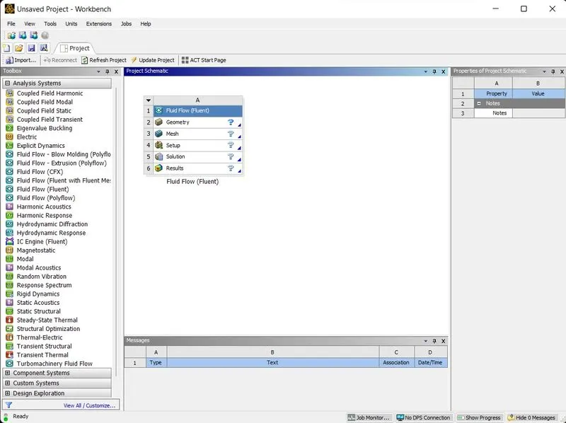
As shown above, these steps are - Geometry and Mesh (Pre-processing), Setup and Solution (Processing) and Results (Post-processing). First, we click on Geometry and the software initiates SpaceClaim which is a CAD cleanup software. Here we can open our design and check for any rough edges, open contours, etc and make ready our design for the simulation. Given that the design imported (short Mixing Tee for the first simulation) is a solid volume, we have to prepare the model such that we retain only the fluid volume. Since this is only a fluid simulation we will not be retaining the solid surfaces. For this we use the command Volume Extract under the Prepare feature in SpaceClaim software. Also to make sure the solid model is not involved in the simulation we hide and use the option suppress for physics on the solid model. 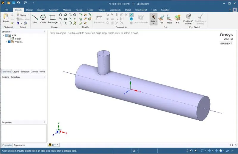
Once the design is ready for the simulation, we close SpaceClaim and enter the next step - Mesh. In the Mesh software, we first label the faces as required - inlet-X, inlet-Y and outlet-X. Then we generate a Mesh over the fluid volume and the parameters are set by Ansys Fluent as per the Bounding Box dimensions. These pre-set mesh parameters are used for the simulation initially. After generating a mesh, we insert a sectional plane along the Z-axis bisecting the fluid volume so as to observe the Meshing performed internally. 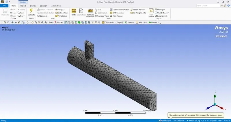
After having checked the Mesh thoroughly, we close the Mesh and click on Setup on the Workbench. This launches Ansys Fluent. In Ansys Fluent, we first have to check for the Mesh quality and if there any errors displayed in the Console we have to go back to Mesh and redefine the Mesh. If there are no errors displayed, then we may go forward with setting up the Physics of the simulation. Here we choose a steady pressure-based solver since the Mach Number is not high. Also since we are solving for Temperature as well we will make use of Energy Equation too. And choose Absolute for Velocity Formation. As for the model, since we wish to capture turbulence as well, we will be going with k-epsilon model in the realisable form. This here is a RANS (Reynolds Average Navier Stokes) model and the RANS equations are used mainly to describe turbulent flow i.e. they are a form of averaging the Navier-Stokes equations based on the Reynolds Decomposition. The RANS approach is the foundation upon which most turbulence models rely on. 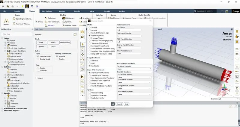
The next thing we need to do is choose the appropriate materials for the fluid volume and we can do this by selecting air from the Fluent Database by opening the Materials panel. Also in this panel, we can also view the properties for the material selected. 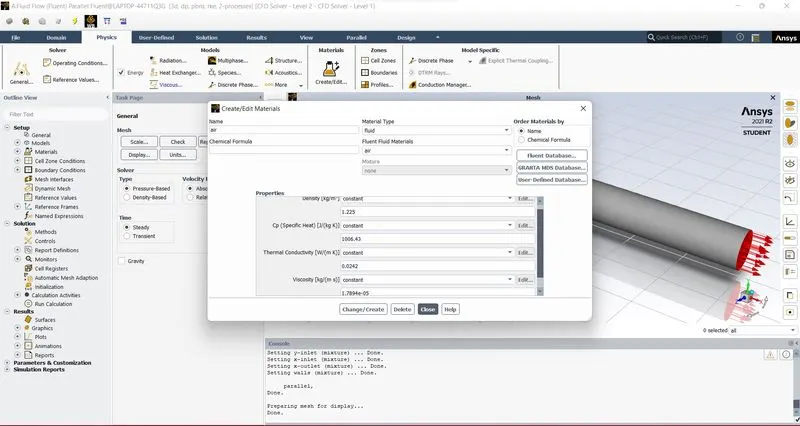
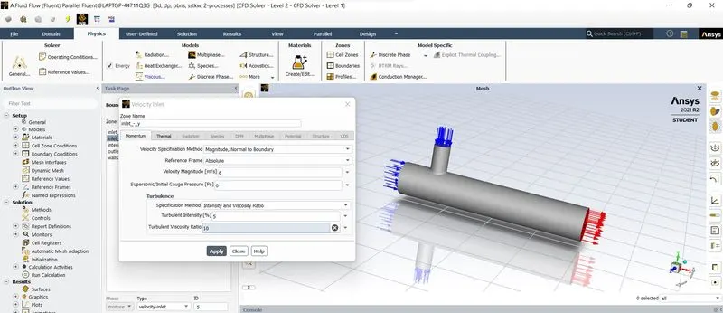
Thus after selecting air as the primary working fluid, we must assign the Boundary Conditions. For this we go to zones and select the cell zones. Here we make sure the material is air thus justifying airflow. Then we go to Boundaries and we redefine the cell boundaries and specify parameters such as Temperature and velocity at the inlets, outlets and the walls. For this we refer to the formulae and the data given in the problem statement. 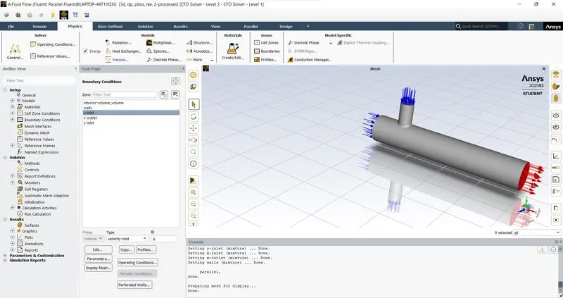
Momentum Ratio = Velocity at cold inlet / Velocity at hot inlet.
Hence, for k-epsilon model the first case:
Case (1a) in a short Mixing Tee with hot inlet of 3m/s velocity and a momentum ratio of 2
`=>` velocity of cold inlet will be 3x2 = 6m/s.
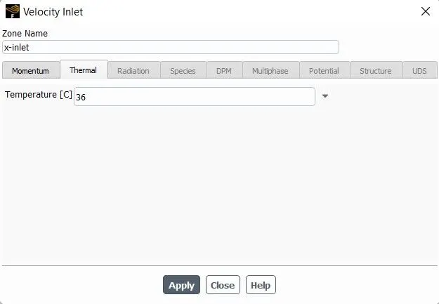
Temperature at cold inlet = 19 deg Celsius
Temperature at hot inlet = 36 deg Celsius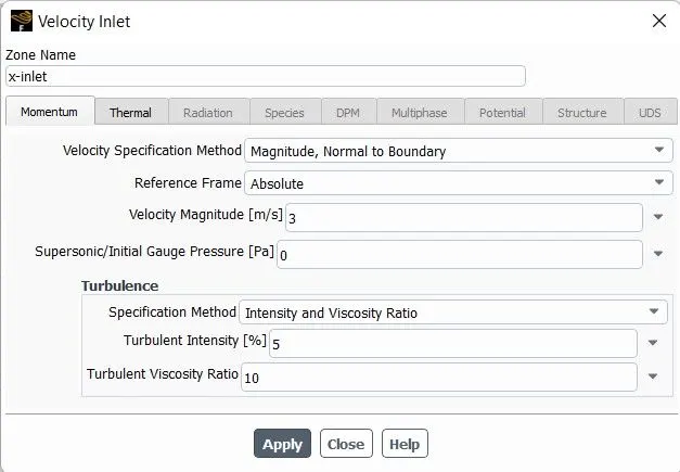
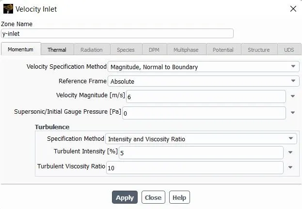
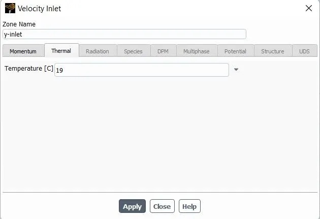
Once the Boundary Conditions are set as required, we need to perform hybrid initialisation (of about 10 iterations) of the simulation. Then we can start the simulations for a set number of iterations (300). 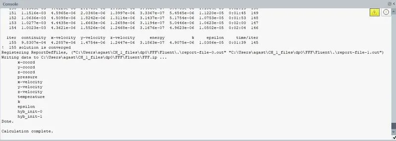
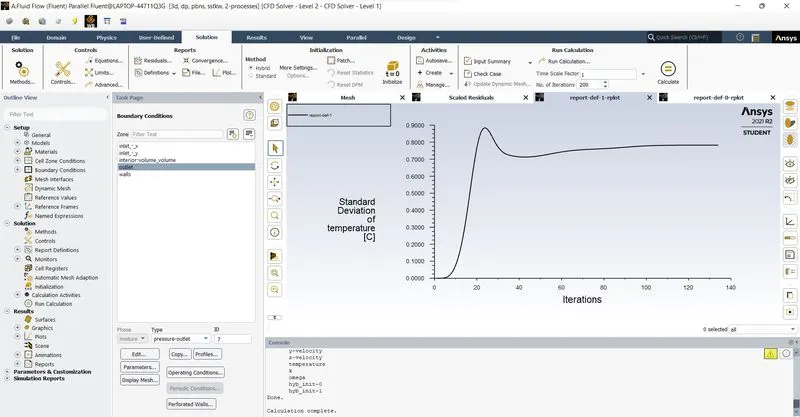
Here in the Console, we observe that solution has attained convergence within 155 trials. 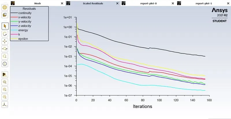
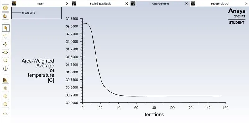
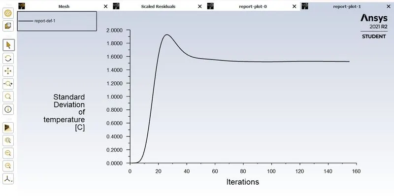
These are the variations of Temperature iteration-wise available in the Ansys Fluent Setup. Once the simulation is complete, we can close the Setup and open the Results in the Workbench for the necessary post-processing.
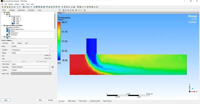
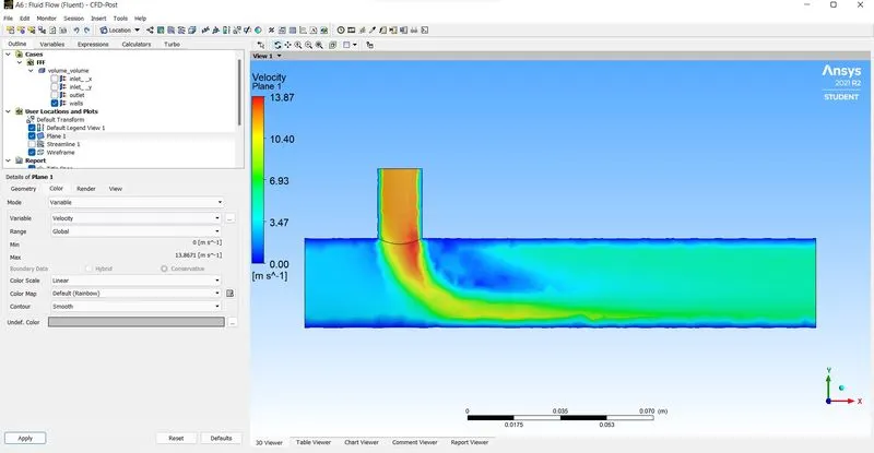
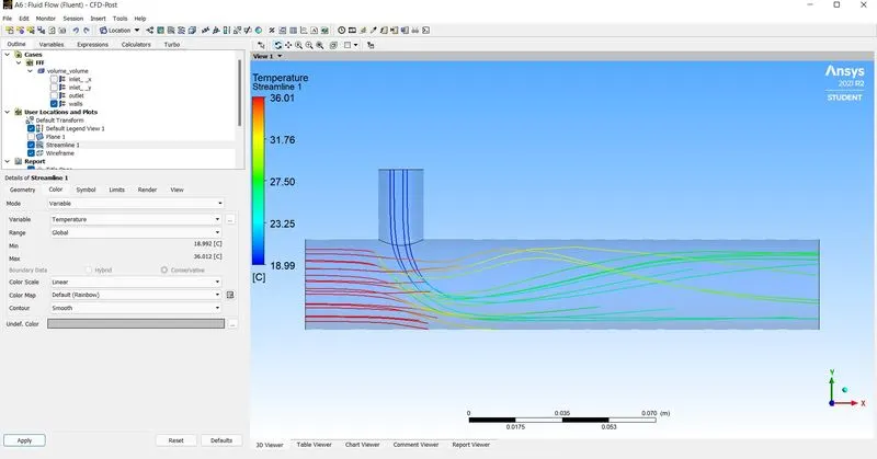
Now that we are back in the workbench we must open the Results for the post-processing. In Results, first we are creating a plane in the z axis coinciding with the axis of the cylinder. Upon this plane we shall plot the distribution of Temperature and also check the changes in Velocity along the axis of the pipe. 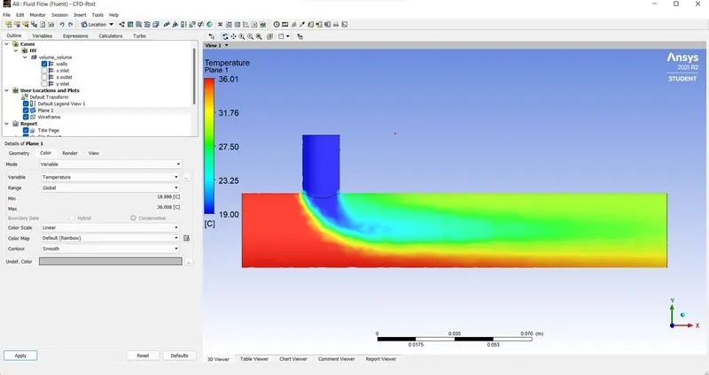
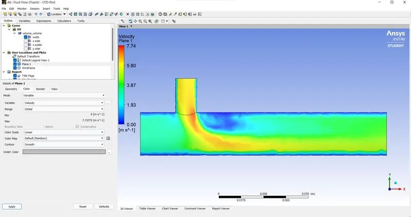
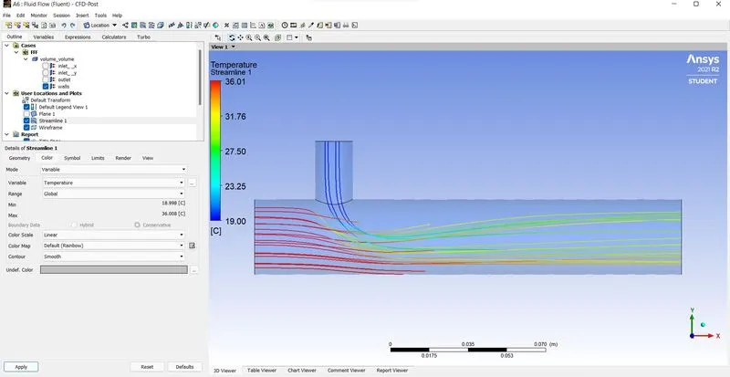
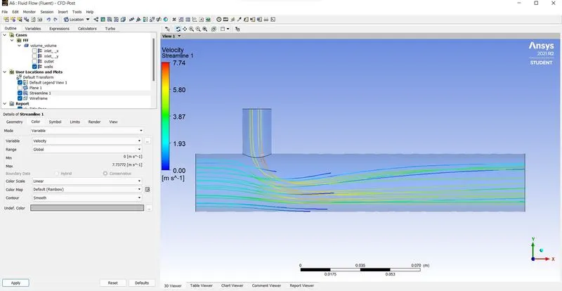
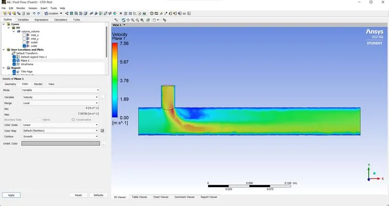
The contour plots attached above, help us visualize the temperature distribution and the velocity changes throughout the plane considered. Similarly, we shall conduct the simulation for the other cases specified:
Case (1b) In a short Mixing Tee with hot inlet of 3m/s velocity and a momentum ratio of 4
`=>` velocity of cold inlet will be 3x4 = 12m/s.
Temperature at cold inlet = 19 deg Celsius
Temperature at hot inlet = 36 deg Celsius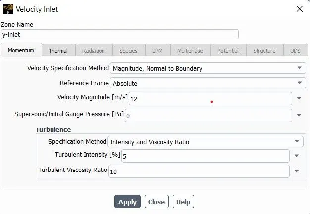
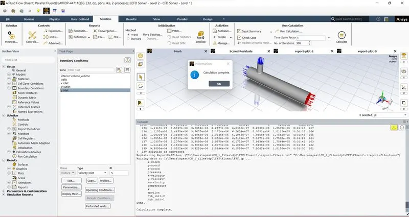
Here in the Console, we observe that solution has attained convergence within 139 trials.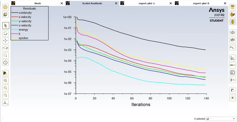
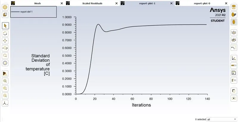
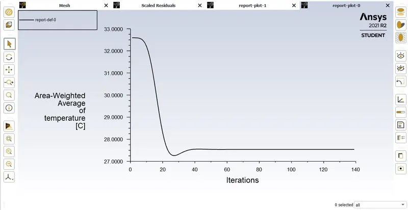
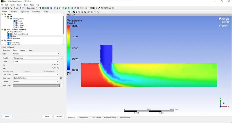
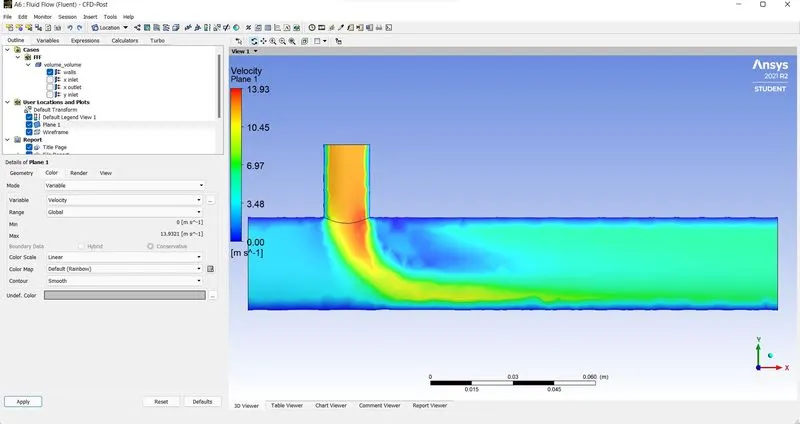
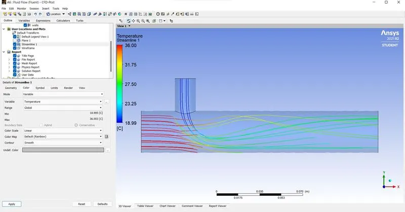
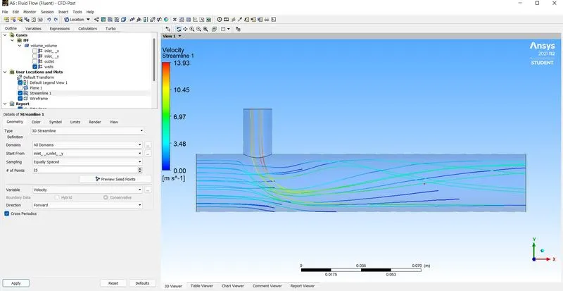
Comparing the above two cases, we get the following data:
| Momentum Ratio | 2 | 4 |
| Cell Count | 12444 | 12444 |
| Average Outlet Temperature (C) | 30.20 | 27.5 |
| Number of iterations for convergence | 155 | 139 |
Now we can simulate the above two cases using k-omega SST model
Hence, for k-omega SST model the first case:
Case (1a) in a short Mixing Tee with hot inlet of 3m/s velocity and a momentum ratio of 2
`=>` velocity of cold inlet will be 3x2 = 6m/s.
Temperature at cold inlet = 19 deg Celsius
Temperature at hot inlet = 36 deg Celsius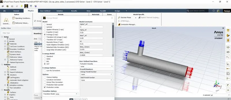
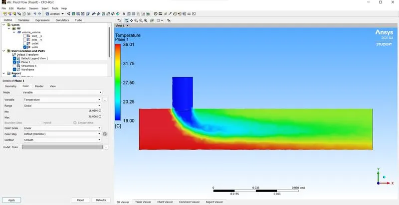
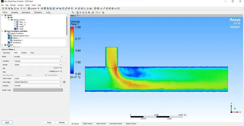
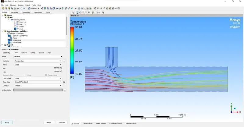
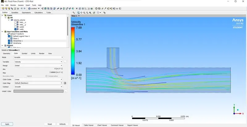
Hence, for k-omega SST model the second case:
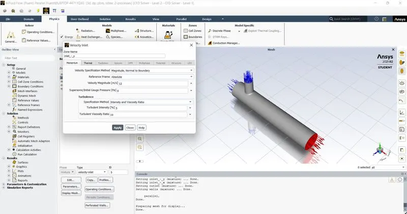
Case (1b) in a short Mixing Tee with hot inlet of 3m/s velocity and a momentum ratio of 4
`=>` velocity of cold inlet will be 3x4 = 12m/s.
Temperature at cold inlet = 19 deg Celsius
Temperature at hot inlet = 36 deg Celsius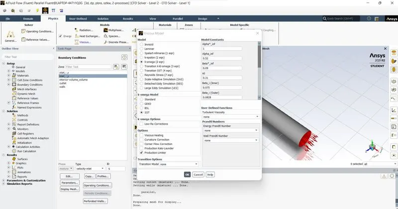
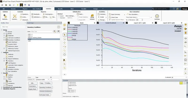
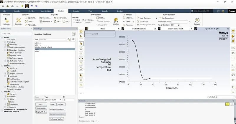
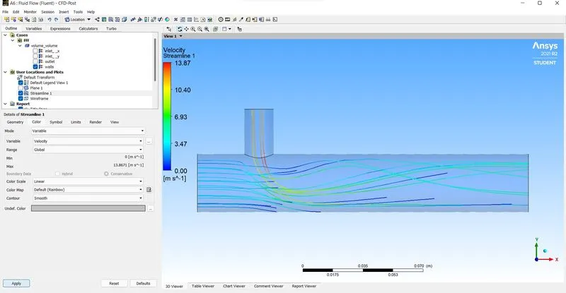
Comparing the above the above two cases, we get the following data:
| Momentum Ratio | 2 | 4 |
| Cell Count | 12444 | 12444 |
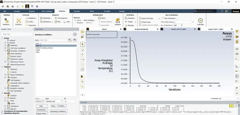
| Average Outlet Temperature [C] | 30.25 | 27.5 |
| Number of iterations required to attain convergence | 160 | 139 |
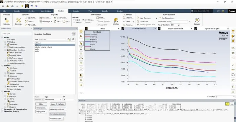
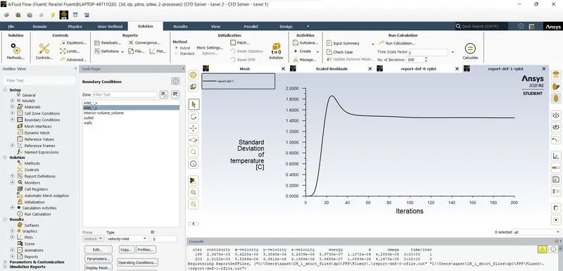
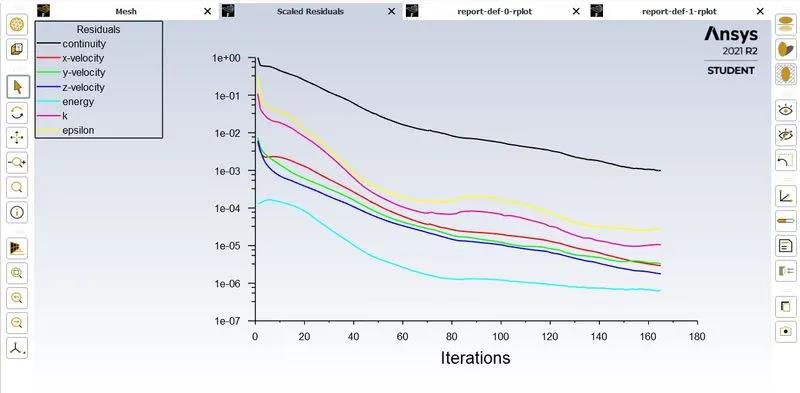
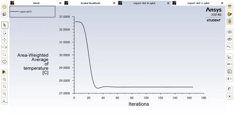
Here, we determine that convergence is attained by observing the variations in the following quantities - the residuals, solution imbalances (mass, momentum and energy) and most importantly the area-weighted average of Temperature. We know that k-epsilon model is best suited for flow away from the wall (free surface flow), whereas k-omega model is best suited for flow near the wall region, where adverse pressure gradient is created.
The baseline k-`epsilon` two-transport-equation model solves for the kinetic energy k and turbulent dissipation `epsilon`. Turbulent dissipation is rate at which velocity fluctuations dissipate. This is very important because these velocity fluctuations directly influence the temperature fluctuations. Thus, turbulent dissipation `epsilon` also helps us determine any thermal stripping occurring in our case. The standard k-`omega` model is a two-transport-equation model that solves for turbulent kinetic energy k and turbulent frequency `omega`. Shear Stress Transport (SST) k-`omega` model is a variant of the standard k-`omega` model that combines the original k-`omega` model and the k-`epsilon` model away from the walls and the eddy viscosity formulation is modified to account for the transport effects of principal turbulent shear stress.
However, taking into account the fact that k-`epsilon` model has comparatively lesser computational requirements and also that k-`omega` models require better mesh resolution at the walls we can choose the k-`epsilon` model in its realisable form since we are only concerned with the internal flow (and hence only the internal flow simulation). Also, since we are concerned only about the thermal mixing at the T-section, the k-`epsilon` model will do for the second case.
Long Mixing Tee
Now we shall simulate a similar situation in a Long Mixing Tee using realisable k-`epsilon` model.
Case (2a) In a Long Mixing Tee with hot inlet of 3m/s velocity and a momentum ratio of 2
`=>` velocity of cold inlet will be 3x2 = 6m/s.
Temperature at cold inlet = 19 deg Celsius
Temperature at hot inlet = 36 deg Celsius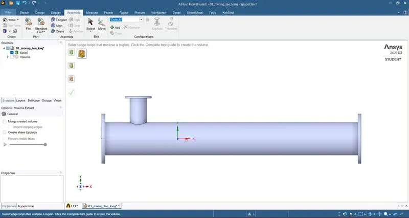
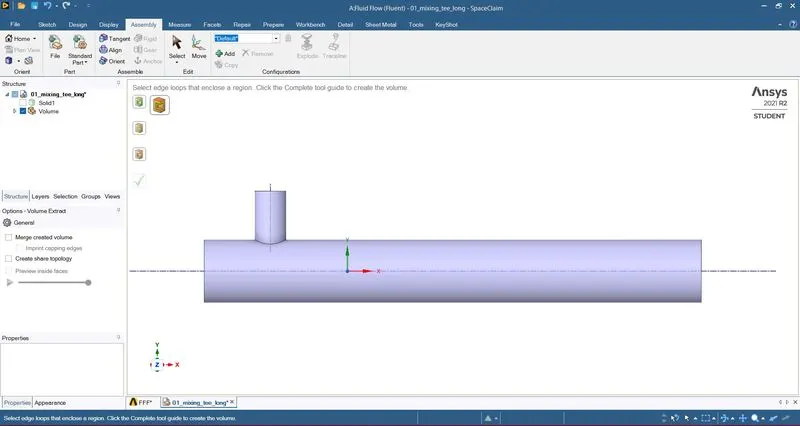
The design is extracted from the given solidworks file and checked in SpaceClaim. The work volume is then extracted as required. 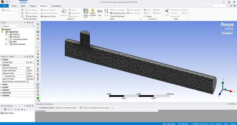
A mesh is applied over the work volume as before and we head forward to the Setup application in Ansys Fluent. 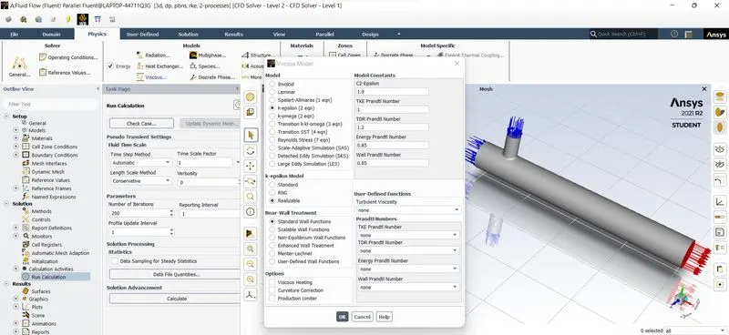
In the Setup application of Ansys Fluent, we setup conditions similar to the case (1a) using k-epsilon model in the realisable form and the rest of the conditions are the exact same as in case (1a). The only difference being the geometry. The case is initialised and then solved as before.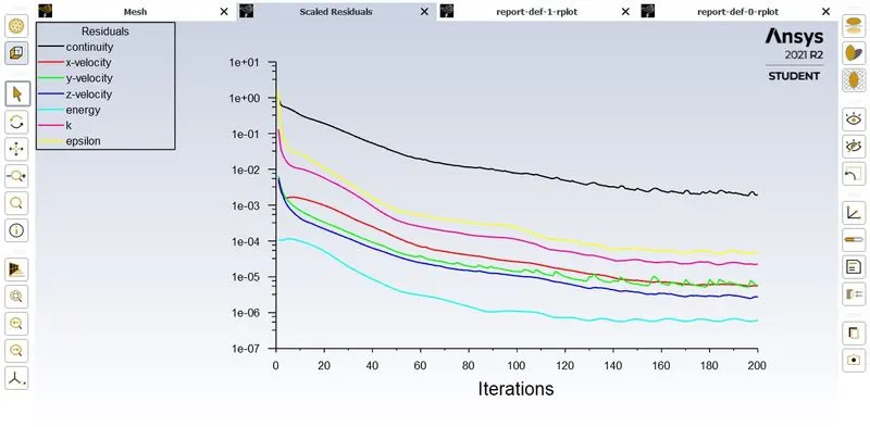
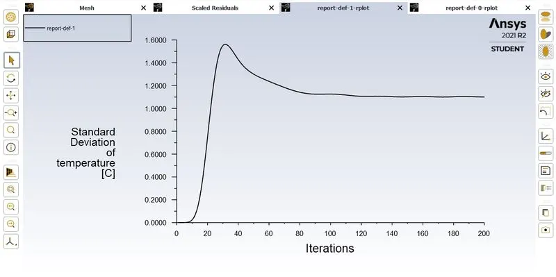
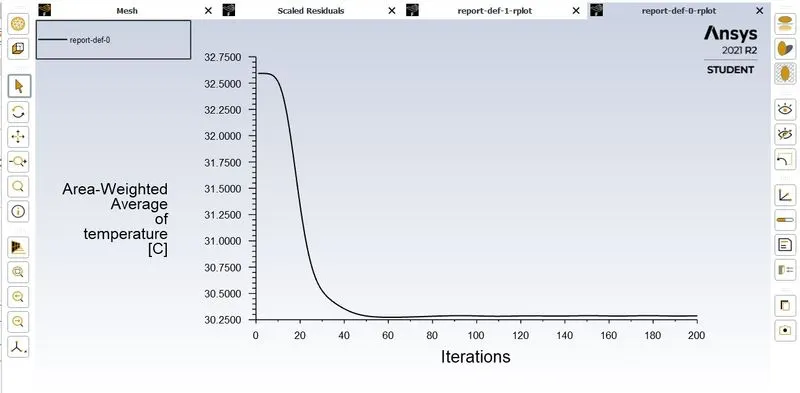
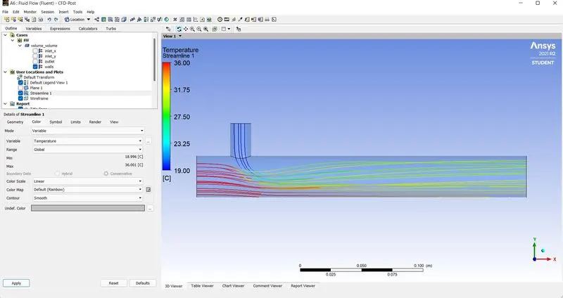
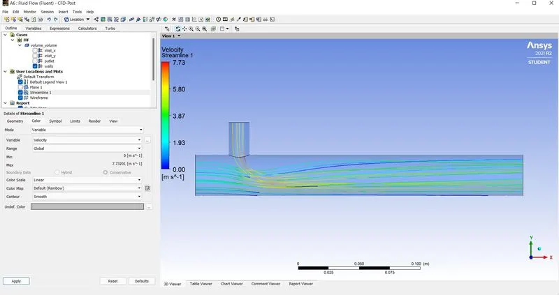
Once the solution is obtained, the required post-processing is done. The results obtained are analysed in CFD-Post. 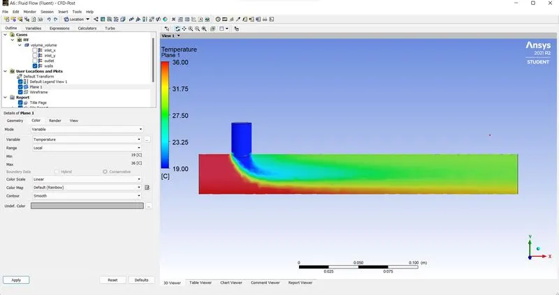
Now that we have
Case (2b) In a Long Mixing Tee with hot inlet of 3m/s velocity and a momentum ratio of 4
`=>` velocity of cold inlet will be 3x4 = 12m/s.
Temperature at cold inlet = 19 deg Celsius
Temperature at hot inlet = 36 deg Celsius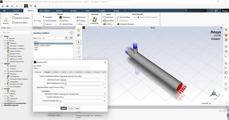
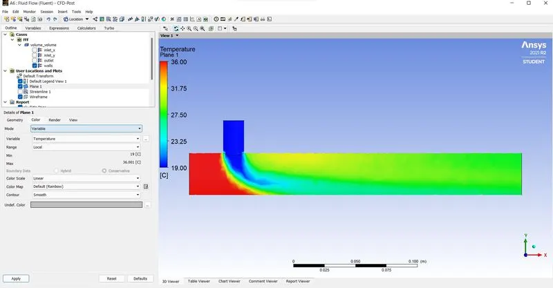
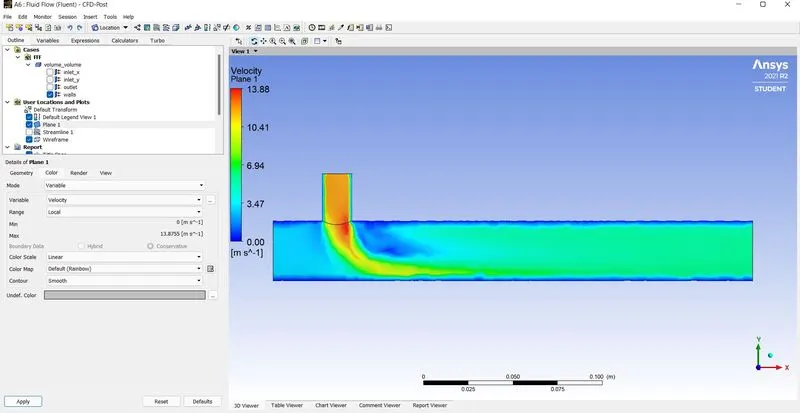
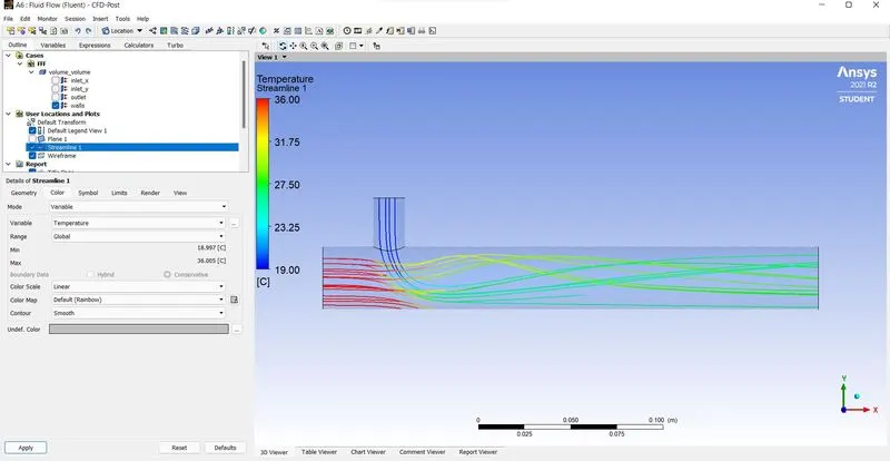
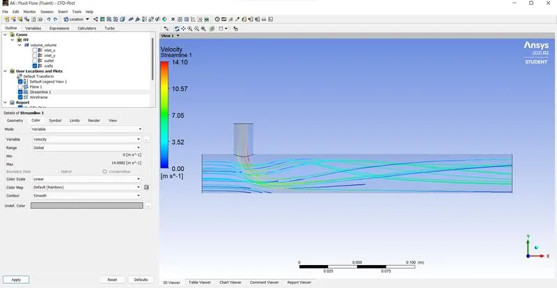
Similar to the comparison in the short mixing tee, we compare the results obtained with each momentum ratio:
| Momentum Ratio | 2 | 4 |
| Cell Count | 15282 | 15282 |
| Average Outlet Temperature [C] | 30.3 | 27.5 |
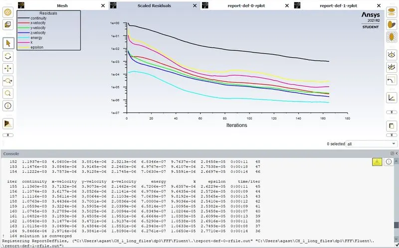
| Minimum number of iterations required to attain convergence | 170 | 164 |
Grid Dependence Test
Here we shall perform a grid independence test on the long mixing tee using k-`epsilon` method in realisable form considering momentum ratio 4.
1) In a Long Mixing Tee with hot inlet of 3m/s velocity and a momentum ratio of 4
`=>` velocity of cold inlet will be 3x4 = 12m/s.
Temperature at cold inlet = 19 deg Celsius
Temperature at hot inlet = 36 deg Celsius
Mesh size `=>` Element Size = 0.01m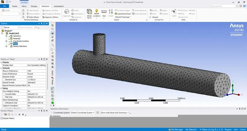
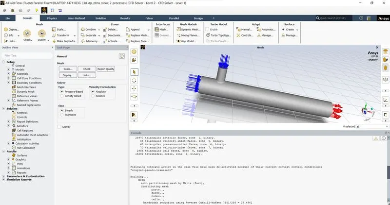
From the console we can observe that with an element size of 0.01m, we get 15282 cells.
Further on we use conditions similar to the case (2b) and we get the following results: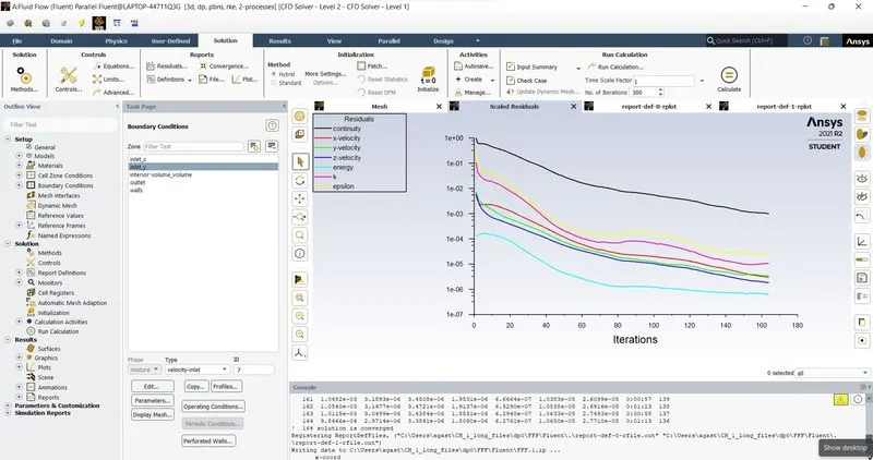
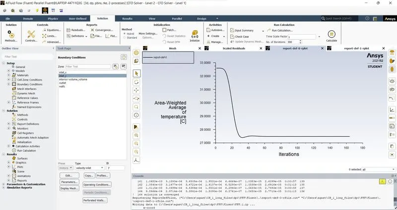
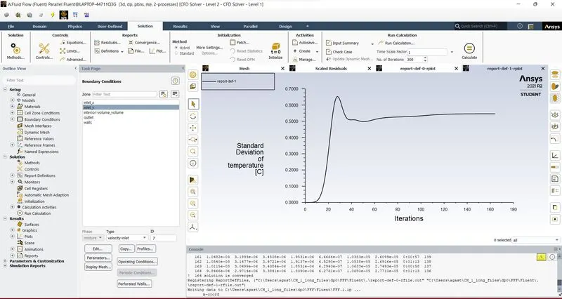
In the Console, we can observe that convergence has been reached after 164 iterations. 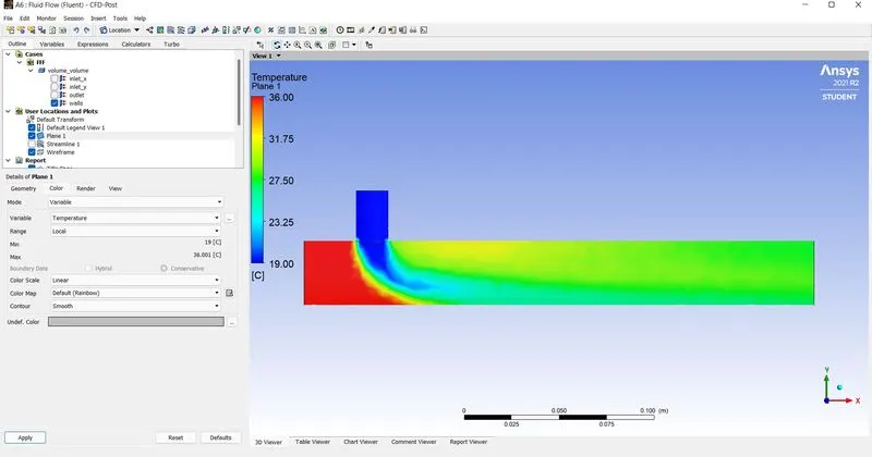
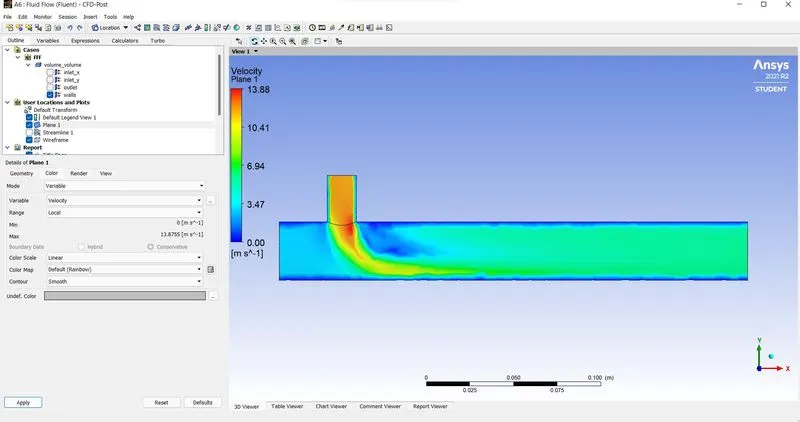
These are the results obtained in CFD-Post.
2) In a Long Mixing Tee with hot inlet of 3m/s velocity and a momentum ratio of 4
`=>` velocity of cold inlet will be 3x4 = 12m/s.
Temperature at cold inlet = 19 deg Celsius
Temperature at hot inlet = 36 deg Celsius
Mesh size `=>` Element Size = 0.005m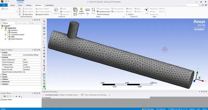
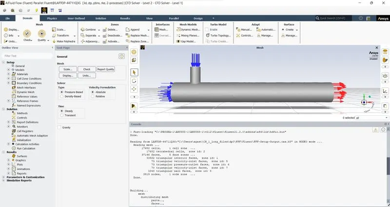
From the console we can observe that with an element size of 0.005m, we get 17682 cells.
Further on we use conditions similar to the case (2b) and we get the following results: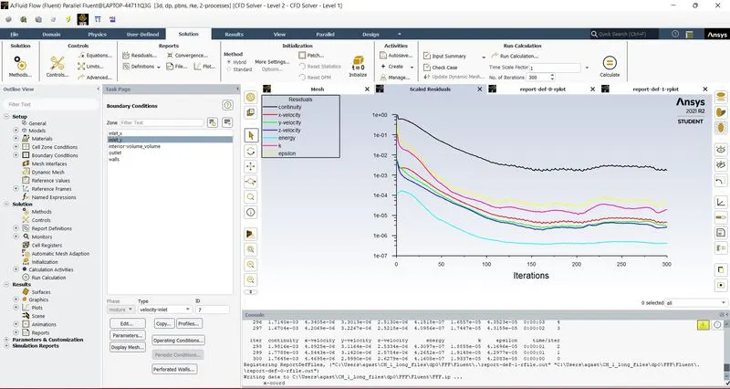
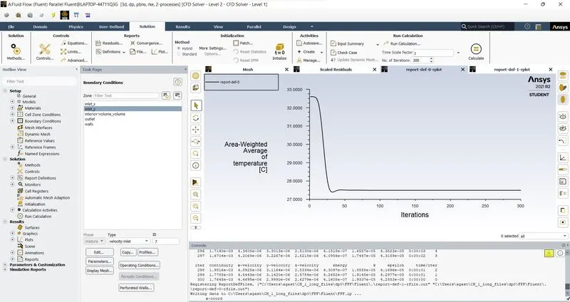
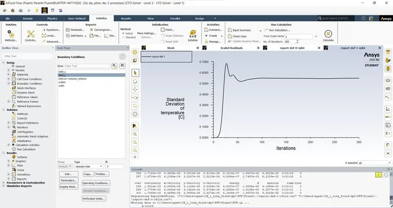
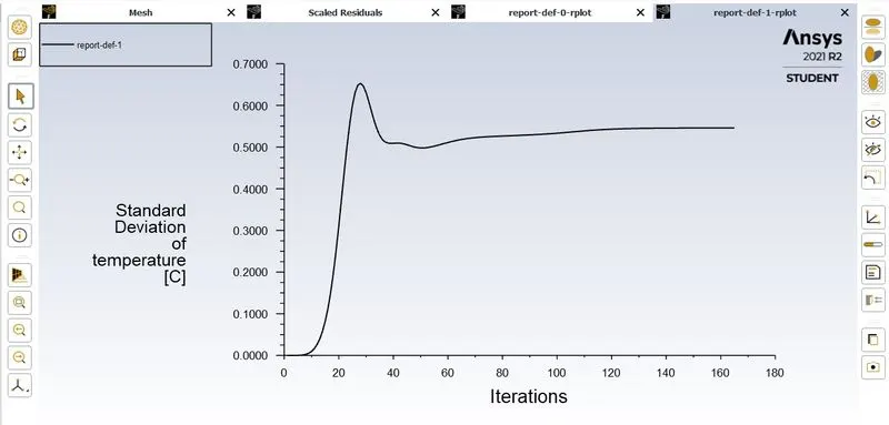
Though convergence has not been indicated in the Console, we can deduce that convergence has been attained by observing the plots indicating the residuals, area-weighted average and standard deviation of Temperature at the outlet face. By further observing these plots, we can also deduce that convergence has been attained after 170 iterations. 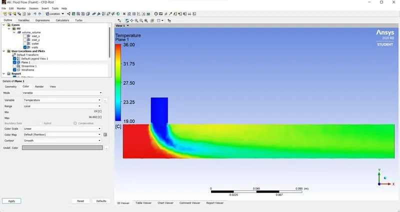
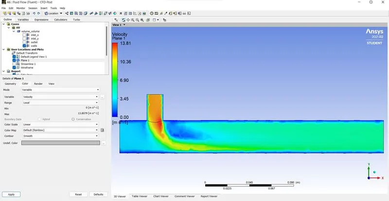
These are the results obtained in CFD-Post.
3) In a Long Mixing Tee with hot inlet of 3m/s velocity and a momentum ratio of 4
`=>` velocity of cold inlet will be 3x4 = 12m/s.
Temperature at cold inlet = 19 deg Celsius
Temperature at hot inlet = 36 deg Celsius
Mesh size `=>` Element Size = 0.002m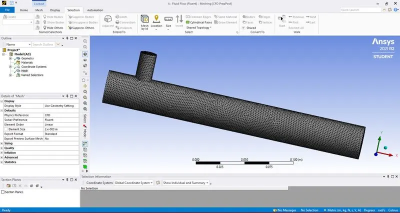
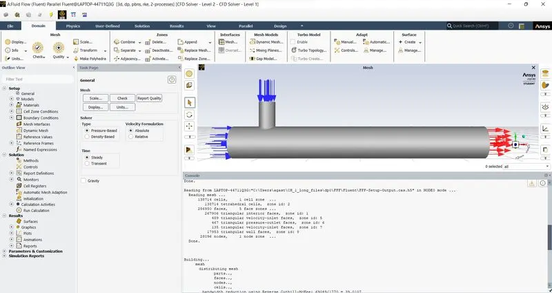
From the console we can observe that with an element size of 0.002m, we get 138714 cells.
Further on we use conditions similar to the case (2b) and we get the following results: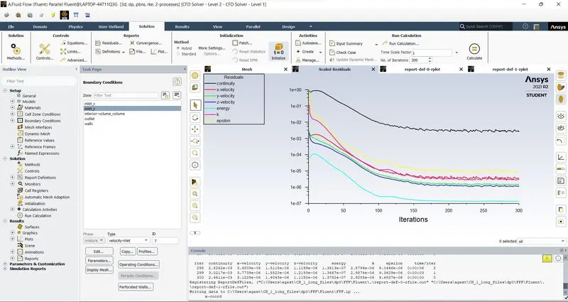
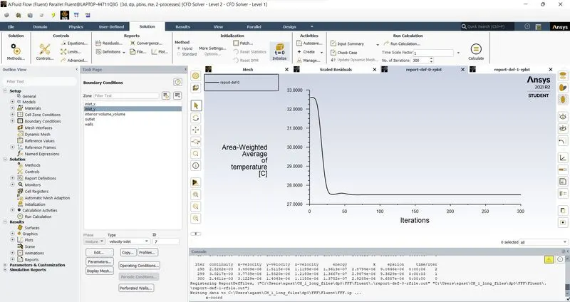
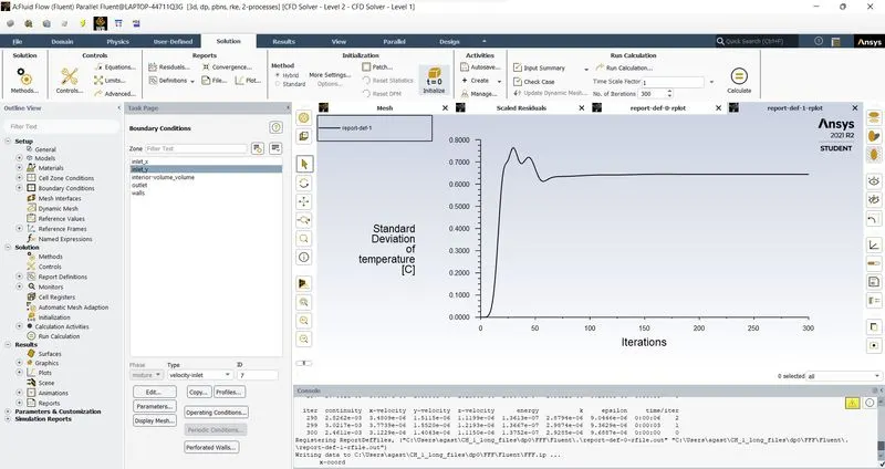
Though convergence has not been indicated in the Console, we can deduce that convergence has been attained by observing the plots indicating the residuals, area-weighted average and standard deviation of Temperature at the outlet face. By further observing these plots, we can also deduce that convergence has been attained after 170 iterations. 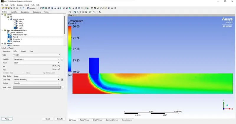
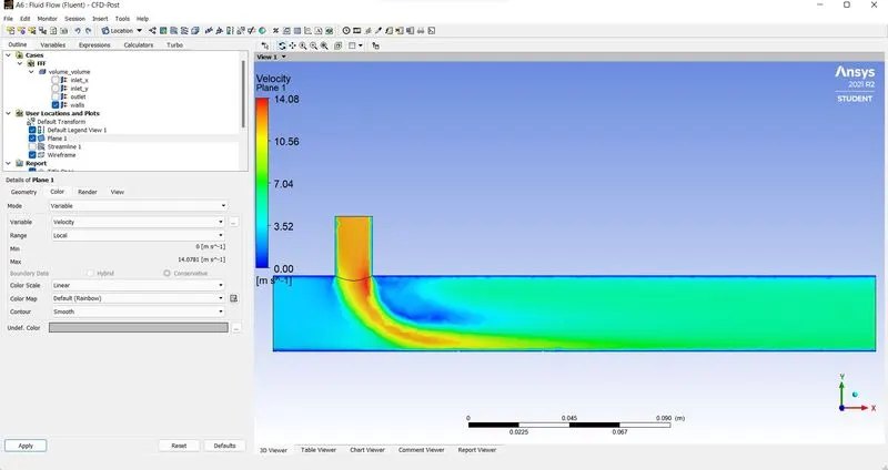
These are the results obtained in CFD-Post.
In these 3 cases, we can observe that the plots representing the Temperature and velocity distributions along the length of the pipe are getting finer and finer as we decrease the element size. This is because the smaller the element size, greater will the number of cells required to encase the total volume under consideration. This can be witnessed in Meshing. And since the number of cells are higher we get greater accuracy, this can also be evidenced by the plots representing the residuals in each of these cases. However, with the extra degree of accuracy we also get a pattern (with very small oscillations) in the residual graphs. This is caused due to the rise of artificial diffusion error. But most importantly , we must also take note of the fact that the quantity under consideration here i.e., Temperature (and velocity) contours similar and show no noticeable difference in the above cases. This implies that the results obtained can be considered true irrespective of the gridsize. Thus, the Grid Dependency Test is performed and this simulation passes the Grid Dependency Test.