Week 1- Mixing Tee
AIM:- To run steady-state simulations of Mixing Tees at different temperatures.
Objective:-
- To understand the mixing effectiveness when hot inlet temperature is 360C & Cold inlet is at 190C.
- Use the k-epsilon and k-omega SST model and conclude the more suitable model.
- The simulation is done for 2cases
Case 1
- Short mixing tee with a hot inlet velocity of 3m/s.
- Momentum ratio of 2, 4.
Case 2
- Long mixing tee with a hot inlet velocity of 3m/s.
- Momentum ratio of 2, 4
Introduction-
Numerical and experimental investigations of mixing in pipelines with side and opposed tees are carried out. Cold fluid flowing in the main pipe is mixed with hot water flowing through a tee. The temperature is measured experimentally to quantify the degree of mixing.
The velocity and temperature fields are also solved numerically. The effects of the mesh size, mesh-localized refinement, dependence of the fluid physical properties on temperature, and turbulence model on numerical results were examined.
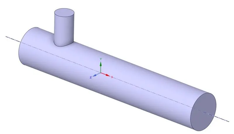
Mixing tee is a flow control device. It mixes the two different fluid streams into a combined fluid stream. It has two inlets and one outlet. In these two inlets, one is located along the X-axis and the other is located along the Y-axis. The outlet is located along the X-axis.
- Computational fluid dynamics (CFD) modeling, such as well-resolved large eddy simulation (LES), can provide accurate predictions of the mixing behavior, including velocity, concentration, and temperature fields, in a mixing tee.
- In this Project we are going to use the ANSYS FLUENT Software to see the mixing effectiveness of two fluids at T- section pipe and these fluids are coming from the different inlets at different temperatures and velocities. The hot inlet Temperature we are going to use is 360C & the Cold inlet is at 190C and for the different velocities, we are going to use momentum ratio.
Momentum ratio = velocity at cold inlet/velocity at hot inlet.
Procedure:-
Step1- Geometry
- In Ansys Fluent we select Fluid Flow(Fluent) for our simulation.
- Then select geometry and Import the Solid Tee CAD file SpaceClaim.
- Then the fluid volume is extracted by using the volume extraction command, Volume extraction is defined as extracting the volume phase from the solid geometry.
- Then hide and suppress for Physics the solid model, It means the solid body is not going to load when we are doing the simulation process.
Step2 - Mesh
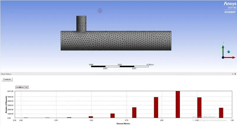
Open Mesh and create the names of the geometry as inlet x, inlet y, outlet, and walls. After this, we are generating mesh and the default mesh size is around mm and we are checking the mesh quality
- Meshing is done by discretizing the solid model into a small element of size 0.004m. We obtained,
No of elements = 22011.
No of nodes = 4759.
Step3 - Setup
Start the Setup in Fluent we have to set up for physics here
- In this case, we are solving for steady-state for small Mach number, and a pressure-based solver is used. Velocity formulations are Absolute and for the Temperature calculation energy equation are used.
- For the Turbulence model in the viscous section, you can use the K- Epsilon and K-omega models as per the equations.
- Now, we are going to add the boundaries values like Velocity and Temperature for the geometry like inlet velocity and inlet Temperature, etc.
- After that, we are going to calculate the average temperature at Outlet and standard deviation for mixing effectiveness of the two fluids at T section by the solution you can get the reports and then initialize the initial conditions and after that hit the calculation we got these reports mentioned below.
- After initialization, a plane has to be created normal to the Z-axis. The temperature and velocity of the Tee are analyzed in the plane and the average temperature at the outlet is to be calculated. Finally, the calculation is to be run for 300 iterations.
Cases
1. For both the models k- Epsilon and k-omega(SST), using momentum ratio is 2 where the hot inlet velocity is 3 m/s and cold inlet velocity 6 m/s
Residual graphs- to check the solution how much numerically accurate
k- Epsilon 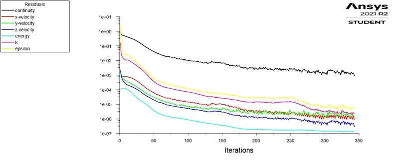 |
k-omega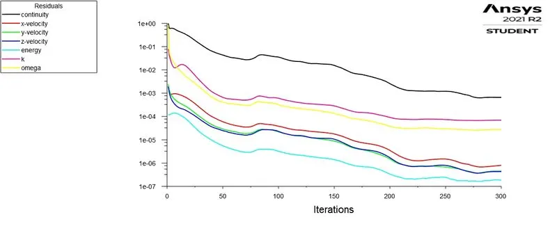 |
Area-weighted graphs Average of Temperature- we use this plot to get the outlet temperature
k- Epsilon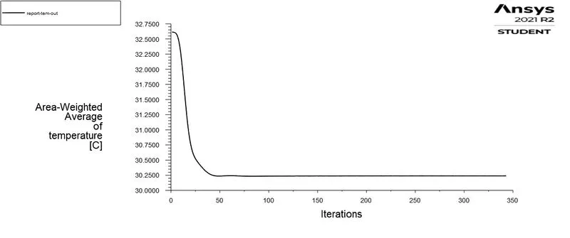 |
k-omega 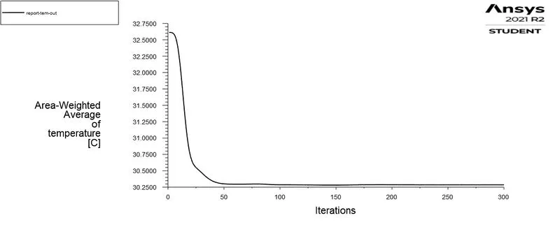 |
Standard Deviation graphs- To understand the effectiveness of mixing.
k- Epsilon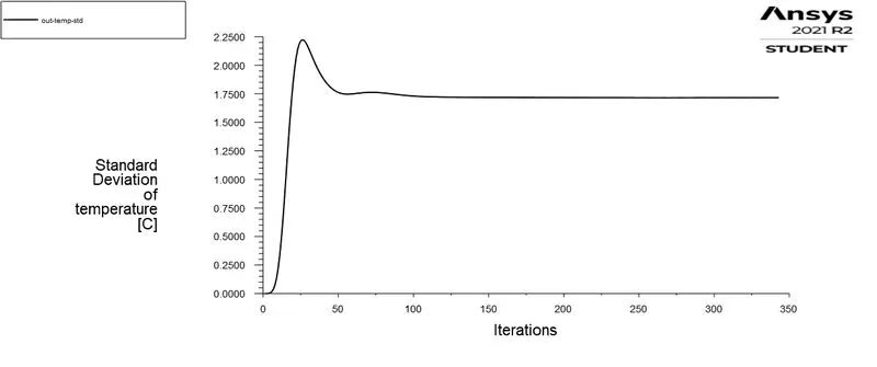 |
k-omega 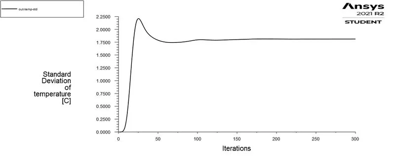 |
Post-processing-
Temperature distribution Along the pipe
k- Epsilon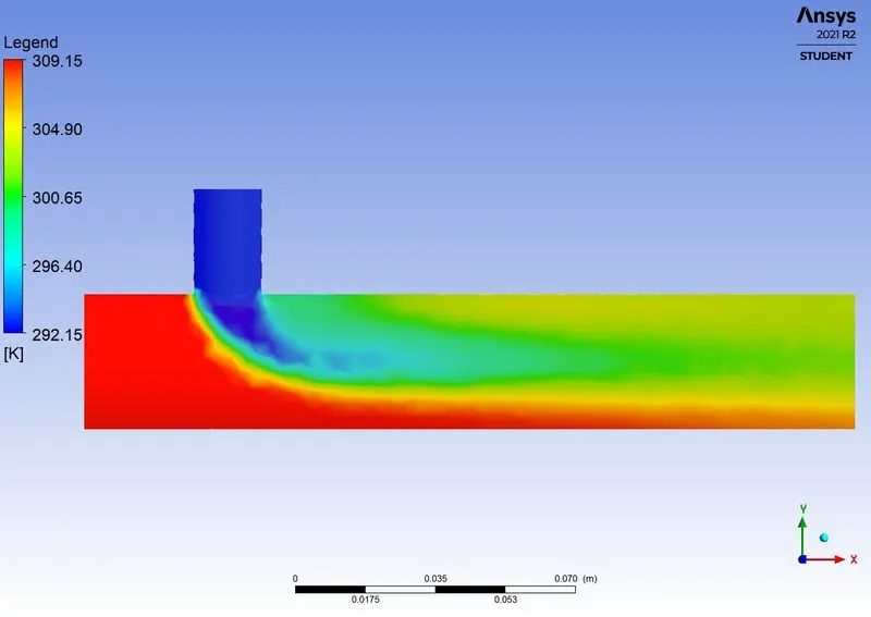 |
k-omega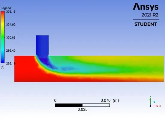 |
Observation:-
- In these plots, we can clearly see that there is a minimum difference between them but In the residual graph, you can clearly see the k-Epsilon model after some value the solution converges and the plot becomes uniform.
- The residual plot always shows a downward slope or decreasing line means the lower the residual value is the more numerically accurate the solution.
- K -Epsilon is used to compute solutions away from the walls and the k-omega model predicts well near walls, each model has certain advantages.
- K- epsilon model shows standard results because it becomes uniform after a certain value So, we are going to use the K-epsilon model for further investigation.
- From the above figures, it is clear that the k-epsilon turbulence model produces a smooth and accurate result than the k-omega SST model.
- From this, we can say that the k-epsilon turbulence model is preferred for further investigation.
2. Mesh Independent study-
In the CFD we have to solve the Governing equations of Fluid dynamics for each cell So, the more cells the more equations we have to solve and that's why it takes time in simulations as per increment in the cell counts. The more the mesh size the cell count number is less and when you decrease the mesh size the cell count is more So, each and every increment of mesh cells you get converged solution means your standard deviation of outlet temperature should reach to steady value as you progressively refining the mesh.
We are going to do Mesh Independent Test for momentum ratio = 2 and using K-Epsilon Turbulence Model
Element Size- 0.004m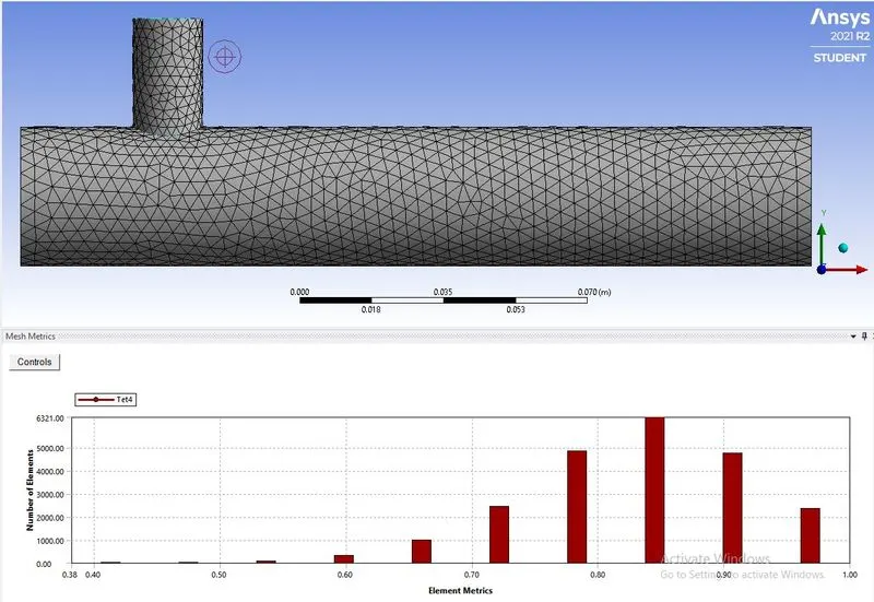 |
Element Size- 0.003m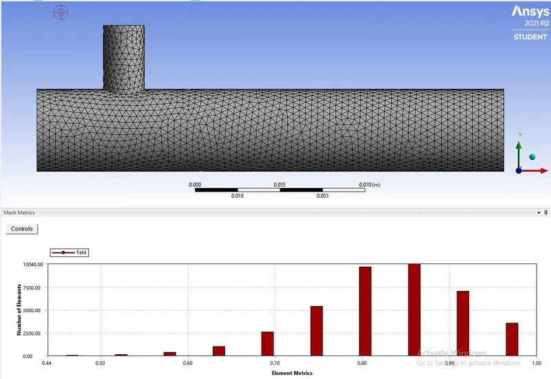 |
Residual graphs- to check the solution how much numerically accurate
| Element Size- 0.004m |
Element Size- 0.003m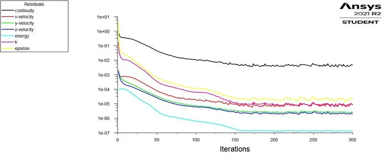 |
Area-weighted graphs Average of Temperature- we use this plot to get the outlet temperature
| Element Size- 0.004m |
Element Size- 0.003m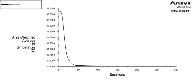 |
Standard Deviation graphs- To understand the effectiveness of mixing.
| Element Size- 0.004 |
Element Size- 0.003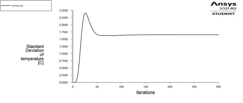 |
Velocity and Temperature along with the pipe contour plots
Temperature Distribution contour plots
| Element Size- 0.004m |
Element Size- 0.003m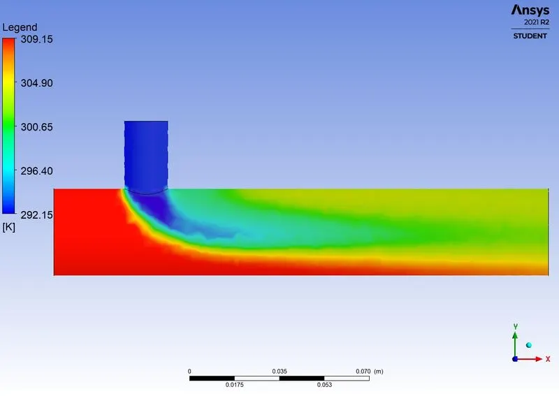 |
Velocity Distribution contour plots
Element Size- 0.004m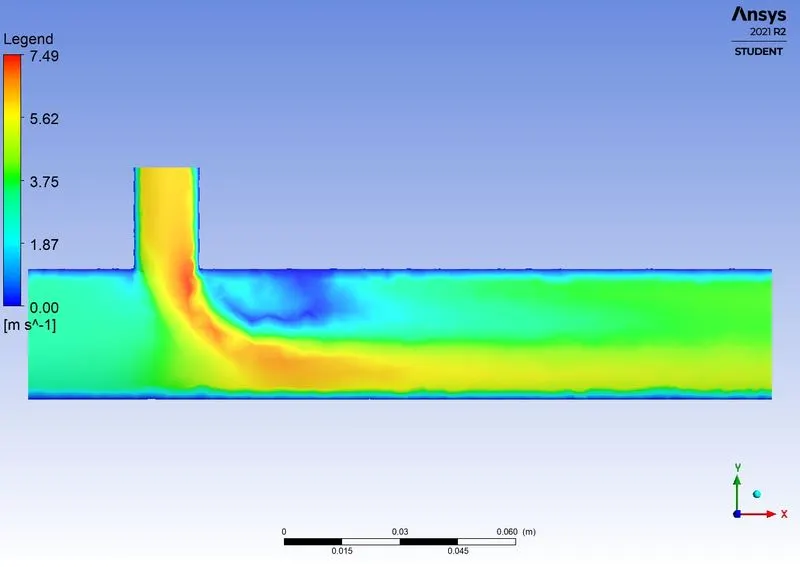 |
Element Size- 0.003m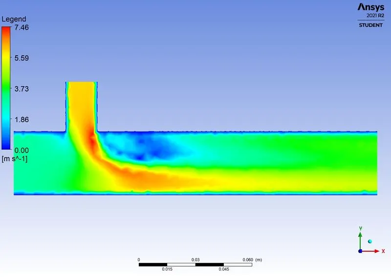 |
Velocity and Temperature across with the pipe contour plots
Temperature Distribution contour plots
Element Size- 0.004m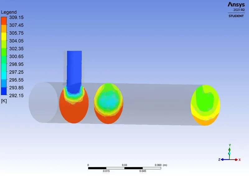 |
Element Size- 0.003m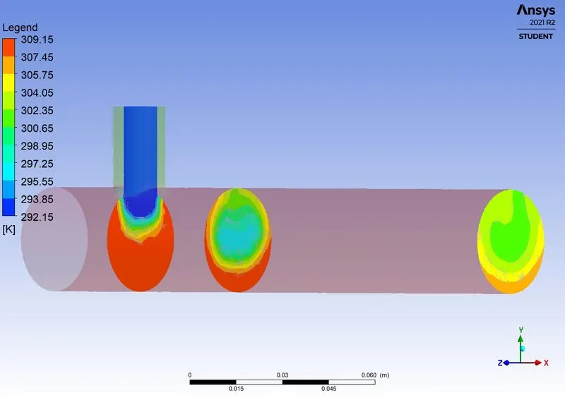 |
Velocity Distribution contour plots
Element Size- 0.004m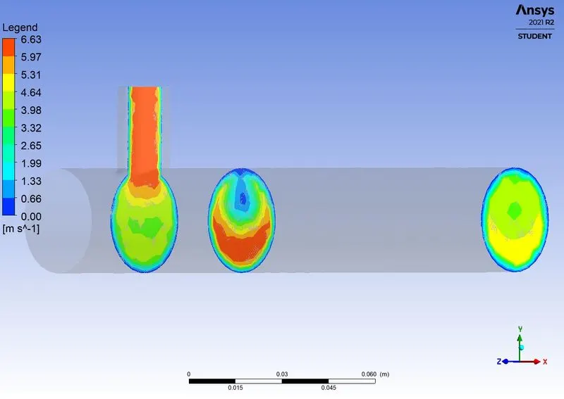 |
Element Size- 0.003m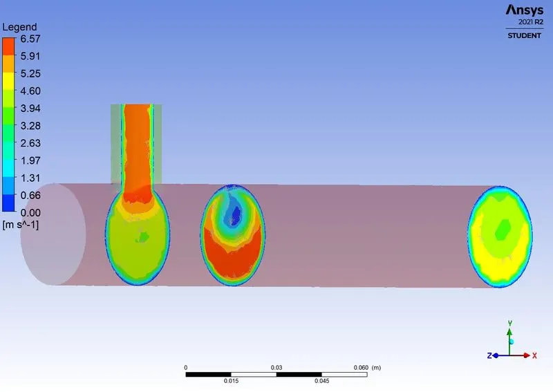 |
Observation-
| cases | Element Size- 0.004m | Element Size- 0.003m |
| Number of Elements | 22011 | 39570 |
| Number of Nodes | 4759 | 8317 |
| Model | K-Epsilon | K-Epsilon |
| No. of Iteration to converge | <300 | <300 |
| Standard Deviation | 1.75 | 1.65 |
- When we increase the number of cells the simulation time increases quadratically. As you add more cells your solver takes more iterations to converge a particular value whereas, If the mesh is coarse (means few cells) the linear solver converges very fast.
- From the above figures, it is clear that the mesh with an element size of 0.003 produces a smooth and accurate result than the mesh with an element size of 0.004.
- From this, we can say that mesh with an Element size of 0.003 is preferred for further investigation.
3. Case1- Short mixing tee
- Short mixing tee with a hot inlet velocity of 3m/s.
- Momentum ratio of 2,4.
- Using the model k- Epsilon, the momentum ratio is 2, so the Hot inlet velocity is 3 m/s and the Cold inlet velocity is 6 m/s and 12m/s.
Output-
Residual graphs- to check the solution how much numerically accurate
| Hot inlet velocity is 3 m/s and Cold inlet velocity is 6 m/s |
Hot inlet velocity is 3 m/s and Cold inlet velocity is 12 m/s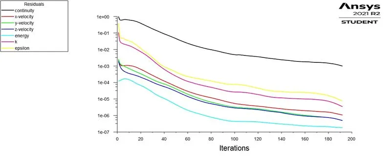 |
Area-weighted graphs Average of Temperature- we use this plot to get the outlet temperature
| Hot inlet velocity is 3 m/s and Cold inlet velocity is 6 m/s |
Hot inlet velocity is 3 m/s and Cold inlet velocity is 12 m/s 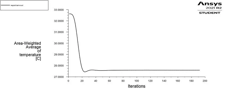 |
Standard Deviation graphs- To understand the effectiveness of mixing.
| Hot inlet velocity is 3 m/s and Cold inlet velocity is 6 m/s |
Hot inlet velocity is 3 m/s and Cold inlet velocity is 12 m/s 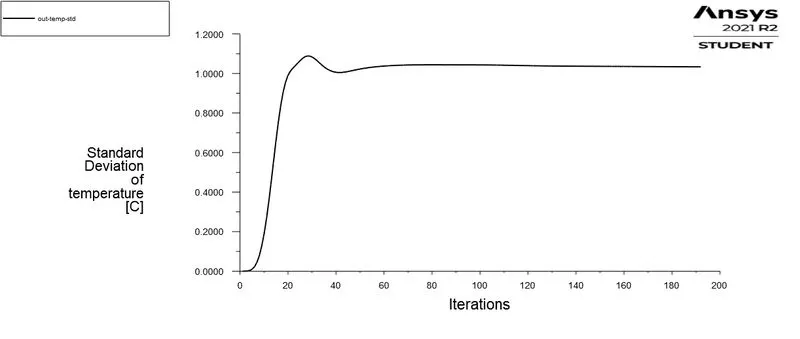 |
Post-processing-
a. Velocity and Temperature along and across the pipe contour plots-
- Velocity and Temperature Contour Plots Along the pipe
Temperature distribution Along the pipe
| Hot inlet velocity is 3 m/s and Cold inlet velocity is 6 m/s |
Hot inlet velocity is 3 m/s and Cold inlet velocity is 12 m/s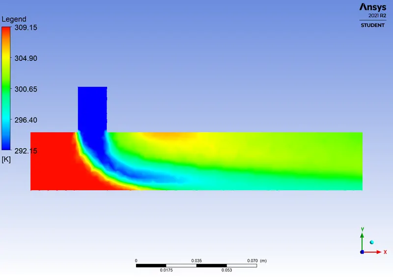 |
Velocity distribution Along the pipe
| Hot inlet velocity is 3 m/s and Cold inlet velocity is 6 m/s |
Hot inlet velocity is 3 m/s and Cold inlet velocity is 12 m/s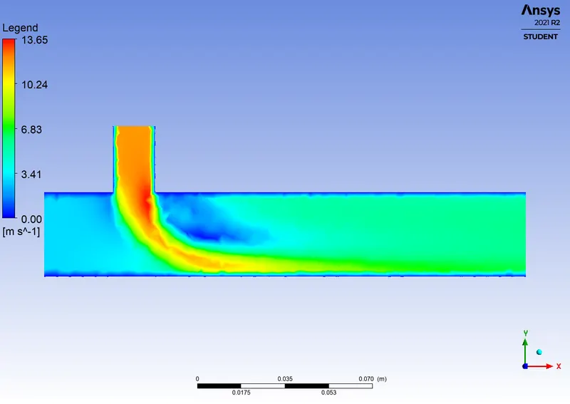 |
- Velocity and Temperature contour plots Across the pipe -
Temperature distribution across the pipe
| Hot inlet velocity is 3 m/s and Cold inlet velocity is 6 m/s |
Hot inlet velocity is 3 m/s and Cold inlet velocity is 12 m/s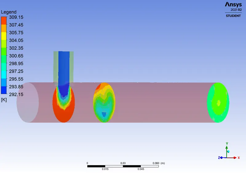 |
Velocity distribution across the pipe
| Hot inlet velocity is 3 m/s and Cold inlet velocity is 6 m/s |
Hot inlet velocity is 3 m/s and Cold inlet velocity is 12 m/s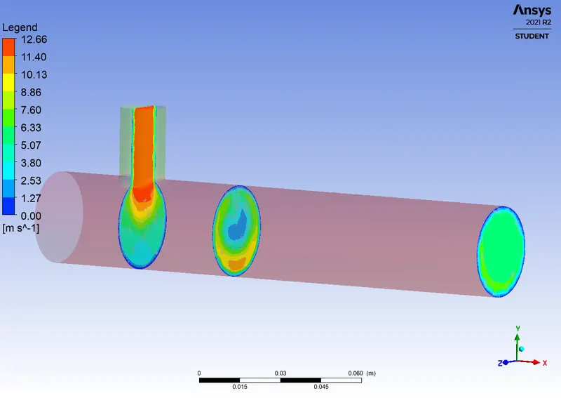 |
b. Velocity and temperature line plots along and across the length of the pipe
- Velocity and Temperature Line Plots Along the pipe
Temperature distribution Along the pipe
Hot inlet velocity is 3 m/s and Cold inlet velocity is 6 m/s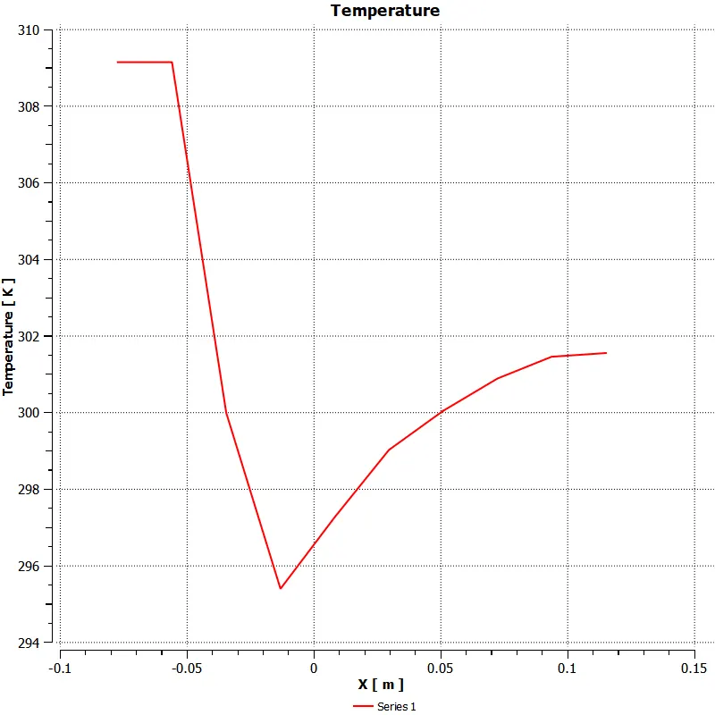 |
Hot inlet velocity is 3 m/s and Cold inlet velocity is 12 m/s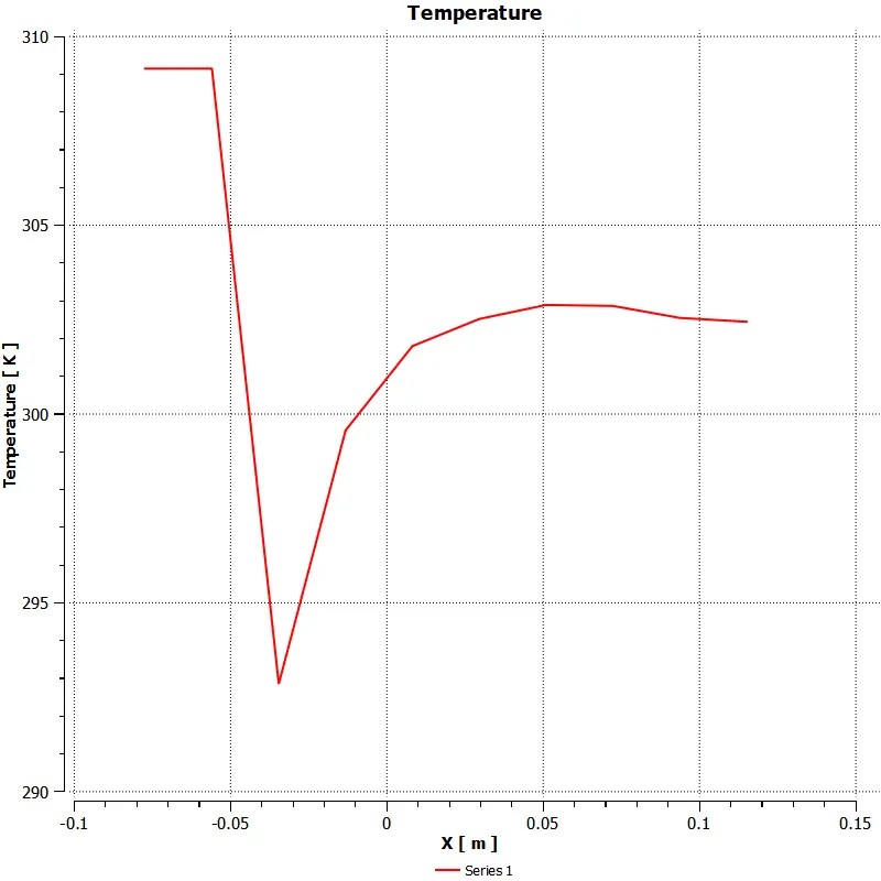 |
Velocity distribution Along the pipe
Hot inlet velocity is 3 m/s and Cold inlet velocity is 6 m/s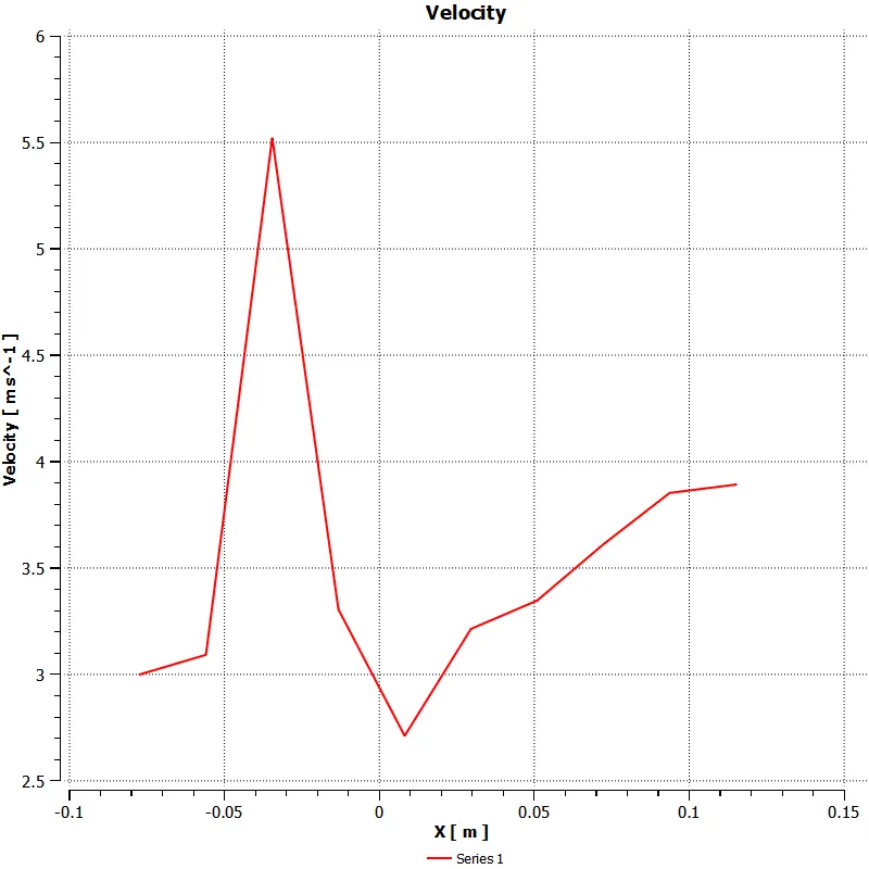 |
Hot inlet velocity is 3 m/s and Cold inlet velocity is 12 m/s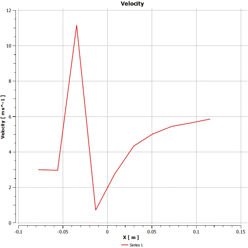 |
- Velocity and Temperature Line plots Across the pipe -
Temperature distribution across the pipe
Hot inlet velocity is 3 m/s and Cold inlet velocity is 6 m/s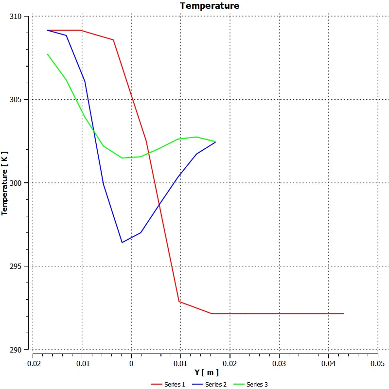 |
Hot inlet velocity is 3 m/s and Cold inlet velocity is 12 m/s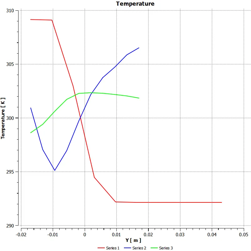 |
Velocity distribution across the pipe
Hot inlet velocity is 3 m/s and Cold inlet velocity is 6 m/s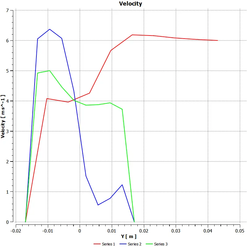 |
Hot inlet velocity is 3 m/s and Cold inlet velocity is 12 m/s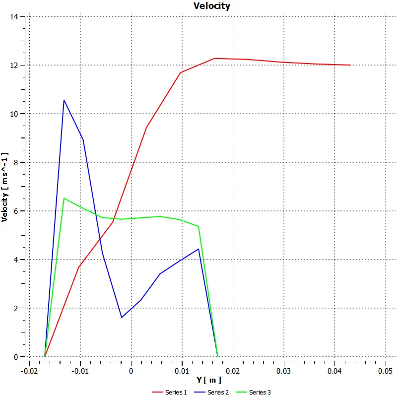 |
Validation-
Formula-
`T_(mixture) = (m_(hot)*T_(hot) + m_(cold)*T_(cold))/(m_(hot) + m_(cold))`
`m_(hot) = rho* A*V_(hot)`
`m_(cold) = rho* A*V_(cold)`
|
Cases |
Hot inlet velocity is 3 m/s and Cold inlet velocity is 6 m/s |
Hot inlet velocity is 3 m/s and Cold inlet velocity is 12 m/s |
|
Analytical Value `T_(mixture)` |
`T_(hot) = 36^o C` `T_(cold) = 19^o C` `A_(hot) = 901.3138 mm^2` `A_(cold) = 225.9823 mm^2` `rho = 1.225 (kg)/m^3` `V_(cold) = 6 m/s` `V_(hot)= 3m/s` `T_(mixture) = 30.3 ^o C` |
`T_(hot) = 36^o C` `T_(cold) = 19^o C` `A_(hot) = 901.3138 mm^2` `A_(cold) = 225.9823 mm^2` `rho = 1.225 (kg)/m^3` `V_(cold) = 6 m/s` `V_(hot)= 12m/s` `T_(mixture) = 27.48 ^o C` |
|
Numerical value `T_(mixture)` |
`T_(mixture) = 30.27 ^o C` |
`T_(mixture) = 27.59 ^o C` |
| Error(%) |
Error = 0.05 |
Error = 0.33 |
| No. of Iteration to converge |
170 |
195 |
- From the above table we can say that the increase in velocity of a fluid is providing a better mixing of temperature at the outlet
4. Case2- Long mixing tee
- Long mixing tee with a hot inlet velocity of 3m/s.
- Momentum ratio of 2,4.
- Using the model k- Epsilon, the momentum ratio is 2, so the Hot inlet velocity is 3 m/s and the Cold inlet velocity is 6 m/s and 12m/s.
Output-
Residual graphs- to check the solution how much numerically accurate
Hot inlet velocity is 3 m/s and Cold inlet velocity is 6 m/s 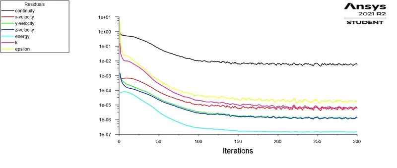 |
Hot inlet velocity is 3 m/s and Cold inlet velocity is 12 m/s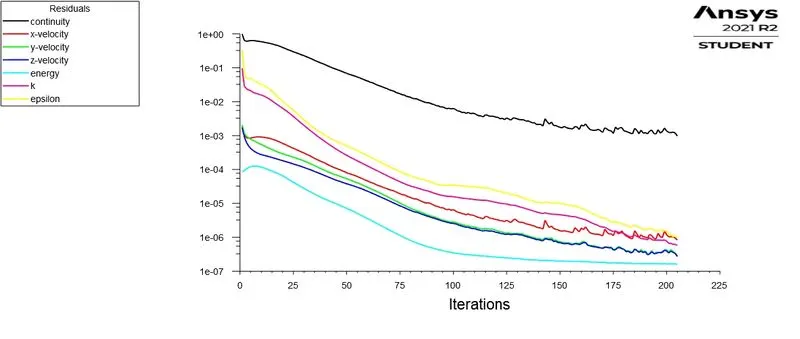 |
Area-weighted graphs Average of Temperature- we use this plot to get the outlet temperature
Hot inlet velocity is 3 m/s and Cold inlet velocity is 6 m/s 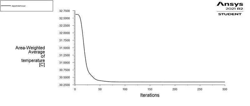 |
Hot inlet velocity is 3 m/s and Cold inlet velocity is 12 m/s 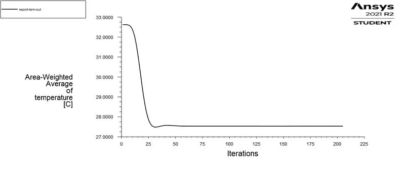 |
Standard Deviation graphs- To understand the effectiveness of mixing.
Hot inlet velocity is 3 m/s and Cold inlet velocity is 6 m/s 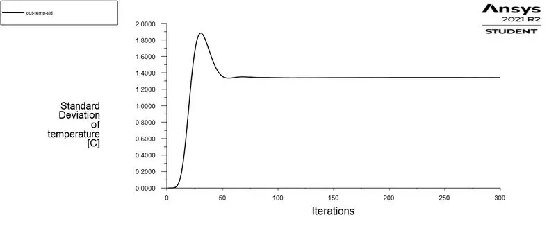 |
Hot inlet velocity is 3 m/s and Cold inlet velocity is 12 m/s 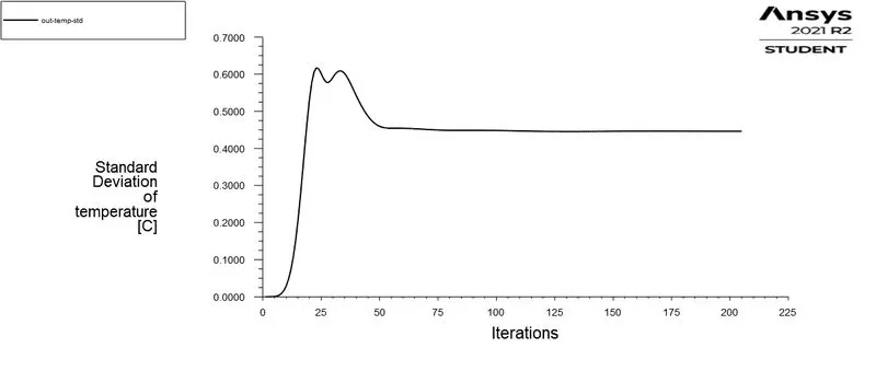 |
Post-processing-
a. Velocity and Temperature along and across the pipe contour plots-
- Velocity and Temperature Contour Plots Along the pipe
Temperature distribution Along the pipe
Hot inlet velocity is 3 m/s and Cold inlet velocity is 6 m/s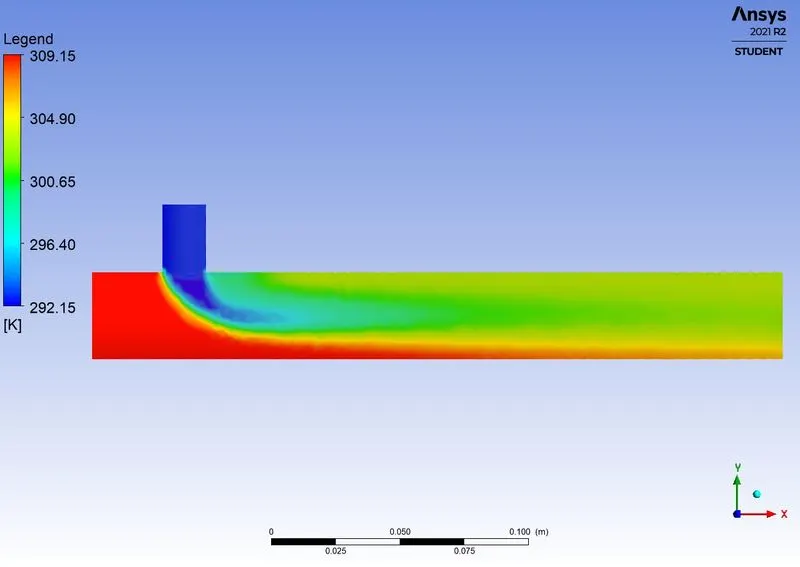 |
Hot inlet velocity is 3 m/s and Cold inlet velocity is 12 m/s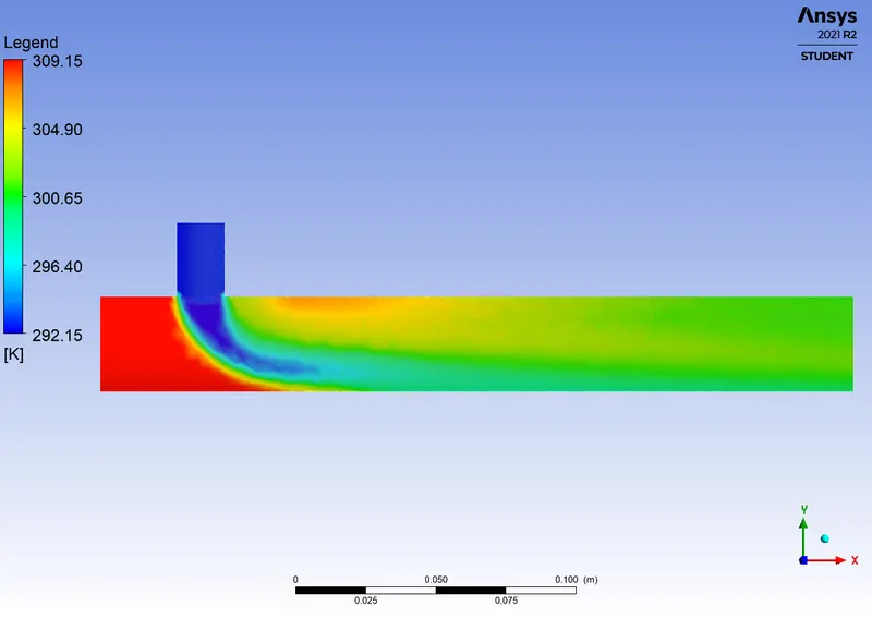 |
Velocity distribution Along the pipe
Hot inlet velocity is 3 m/s and Cold inlet velocity is 6 m/s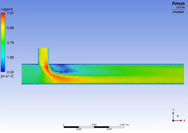 |
Hot inlet velocity is 3 m/s and Cold inlet velocity is 12 m/s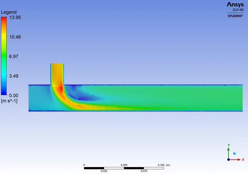 |
- Velocity and Temperature contour plots Across the pipe -
Temperature distribution across the pipe
Hot inlet velocity is 3 m/s and Cold inlet velocity is 6 m/s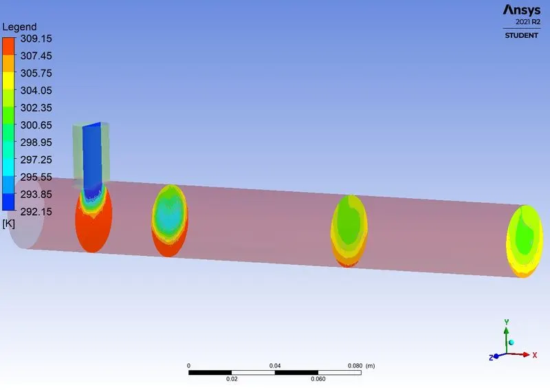 |
Hot inlet velocity is 3 m/s and Cold inlet velocity is 12 m/s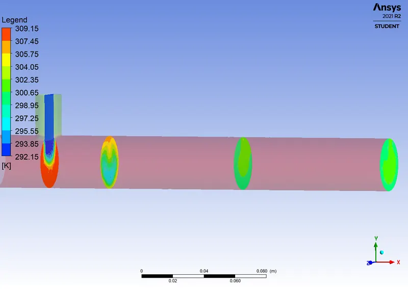 |
Velocity distribution across the pipe
Hot inlet velocity is 3 m/s and Cold inlet velocity is 6 m/s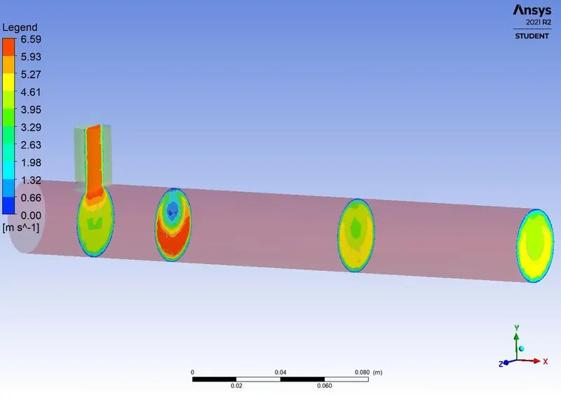 |
Hot inlet velocity is 3 m/s and Cold inlet velocity is 12 m/s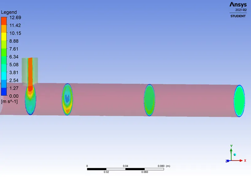 |
b. Velocity and temperature line plots along and across the length of the pipe
- Velocity and Temperature Line Plots Along the pipe
Temperature distribution Along the pipe
Hot inlet velocity is 3 m/s and Cold inlet velocity is 6 m/s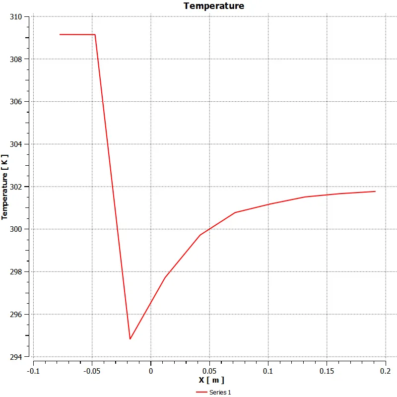 |
Hot inlet velocity is 3 m/s and Cold inlet velocity is 12 m/s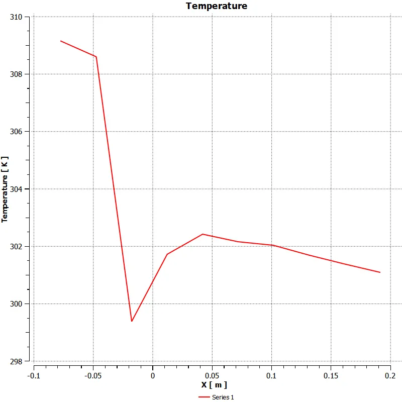 |
Velocity distribution Along the pipe
Hot inlet velocity is 3 m/s and Cold inlet velocity is 6 m/s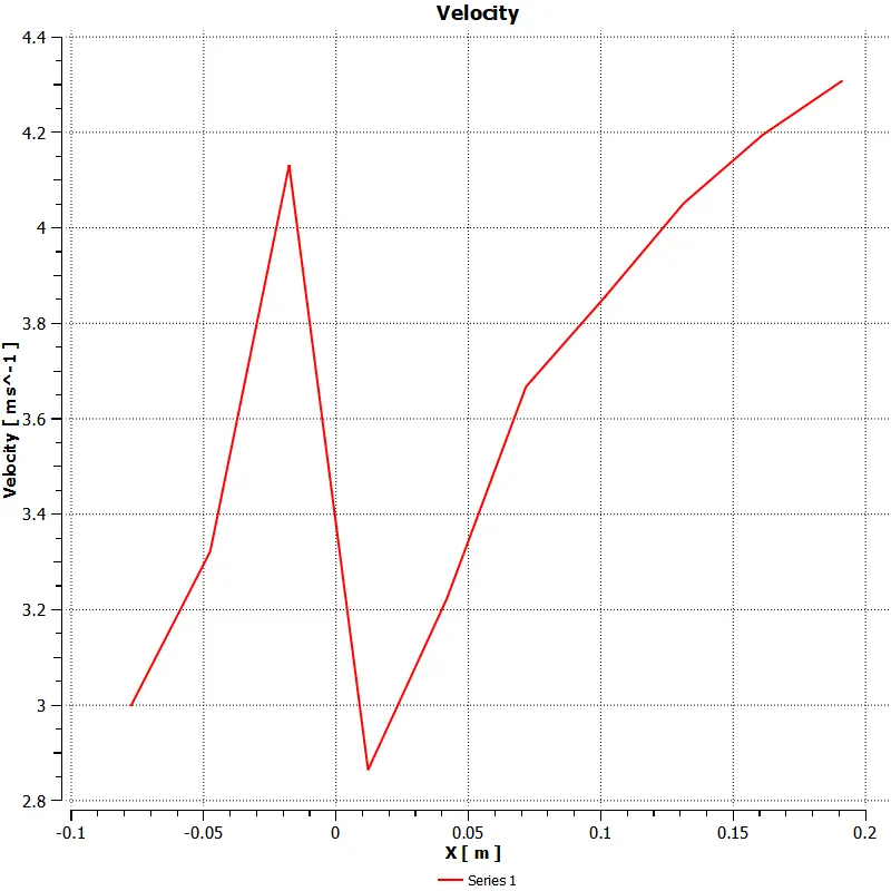 |
Hot inlet velocity is 3 m/s and Cold inlet velocity is 12 m/s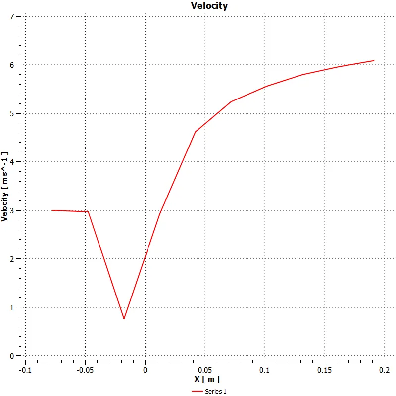 |
- Velocity and Temperature Line plots Across the pipe -
Temperature distribution across the pipe
Hot inlet velocity is 3 m/s and Cold inlet velocity is 6 m/s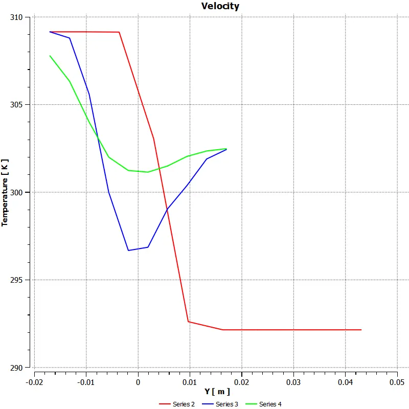 |
Hot inlet velocity is 3 m/s and Cold inlet velocity is 12 m/s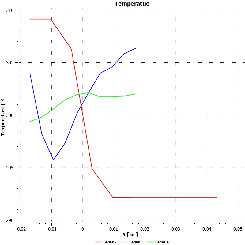 |
Velocity distribution across the pipe
Hot inlet velocity is 3 m/s and Cold inlet velocity is 6 m/s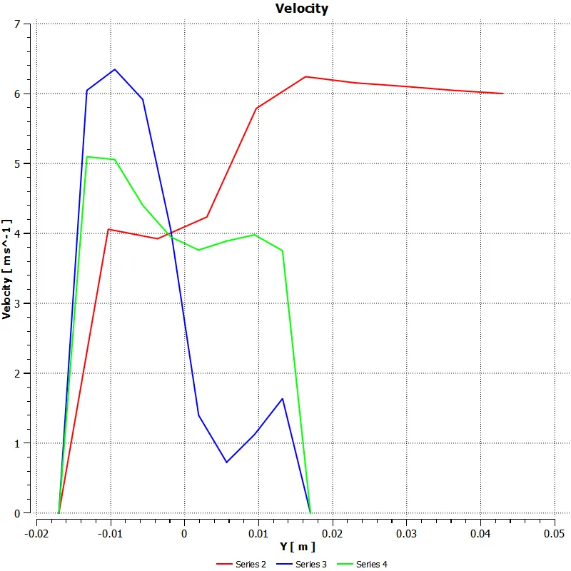 |
Hot inlet velocity is 3 m/s and Cold inlet velocity is 12 m/s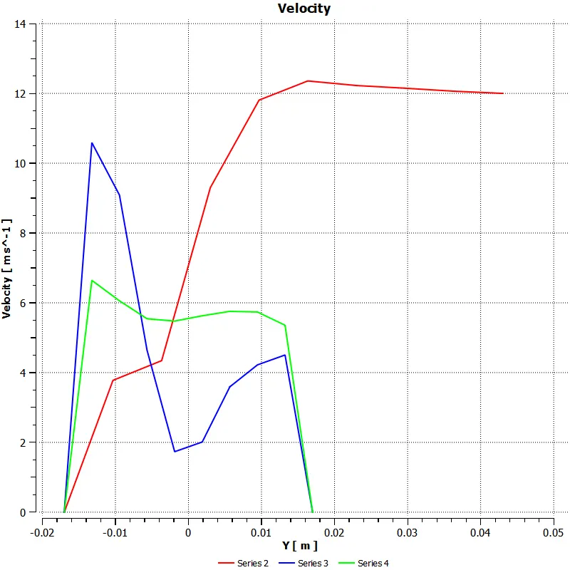 |
Validation-
Formula-
`T_(mixture) = (m_(hot)*T_(hot) + m_(cold)*T_(cold))/(m_(hot) + m_(cold))`
`m_(hot) = rho* A*V_(hot)`
`m_(cold) = rho* A*V_(cold)`
|
Cases |
Hot inlet velocity is 3 m/s and Cold inlet velocity is 6 m/s |
Hot inlet velocity is 3 m/s and Cold inlet velocity is 12 m/s |
|
Analytical Value `T_(mixture)` |
`T_(hot) = 36^o C` `T_(cold) = 19^o C` `A_(hot) = 901.3138 mm^2` `A_(cold) = 225.9823 mm^2` `rho = 1.225 (kg)/m^3` `V_(cold) = 6 m/s` `V_(hot)= 3m/s` `T_(mixture) = 30.3 ^o C` |
`T_(hot) = 36^o C` `T_(cold) = 19^o C` `A_(hot) = 901.3138 mm^2` `A_(cold) = 225.9823 mm^2` `rho = 1.225 (kg)/m^3` `V_(cold) = 6 m/s` `V_(hot)= 12m/s` `T_(mixture) = 27.48 ^o C` |
|
Numerical value `T_(mixture)` |
`T_(mixture) = 30.34 ^o C` |
`T_(mixture) = 27.53 ^o C` |
| Error(%) |
Error = 0.23 |
Error = 0.20 |
| No. of Iteration to converge |
180 |
205 |
- From the above table we can say that the increase in velocity of a fluid is providing a better mixing of temperature at the outlet
Observations from both the cases
- After comparing we can conclude that the increase in length doesn't have any effect on the mixing of temperature at the outlet and increasing the velocity provides better mixing of temperature at the outlet
Conclusion-
- From the Grid independence test, we can conclude that the finer the size of the mesh, the better the accuracy of the solution. This is because if the cell size decreases the error is linearly proportional to the cell size, so the error also decreases. Hence at the finer grid size, we got better mixing efficiency. But at the same time, computational time increases significantly.
- Both K-Epsilon and K-Omega turbulence model was used for the first case and found that outlet temperature was the same but a slight difference in standard deviation was observed.
- But the main difference is that K-Epsilon is used for the analysis of flow away from the walls and K-Omega is used for the analysis of flow near the wall. In our case, we are dealing with the flow away from the wall so K-Epsilon is the suitable turbulence model.
- The velocity, temperature contour along mixing tee shows that a small portion of high-temperature fluid slips at the outlet in case of lower momentum ratio but there is no such slip in case of higher momentum ratio.
- Also in the validation perspective higher momentum ratio results are much closer to the analytical results compared to the lower momentum ratio and more importantly, the mixing effect is better in the case with a higher momentum ratio as the standard deviation value was less.
- Comparing the contours and standard deviation reports of both long and short tee suggests that an increase in length increases the mixing effectiveness.