Week 1- Mixing Tee

AIM: To set up steady-state simulations to compare the mixing effectiveness when hot fluid inlet temperature is 36⁰C & the Cold fluid inlet

is at 19⁰C that flows in a mixing tee.

1. Case 1
   • Short mixing tee with a hot inlet velocity of 3m/s.
   • Momentum ratio of 2, 4.
2. Case 2
   • Long mixing tee with a hot inlet velocity of 3m/s.
   • Momentum ratio of 2, 4.

Momentum ratio = velocity at cold inlet / velocity at hot inlet

In a table, compare the following values from the 2 cases.

1. Cell count
2. Average outlet temperature
3. Number of iterations for convergence

Expected results:

1. Velocity and temperature contour plots on the cut planes along and across the pipe.
2. Velocity and temperature line plots along and across the length of the pipe.
3. Perform Mesh independent study for any one case.
4. Discuss the effect of length and momentum ratio on results.

Introduction

• A mixing Tee is formed by two pipe sections joined at a right angle to each other.
• One stream passes straight through the Tee while other enters perpendicular at one side.
• These are used in blending of some oils(injection of additives) and petro-chemical products.
• Blending of fuel gas and mixing of feed streams for catalytic reactors.
• These are having applications in HVAC system .

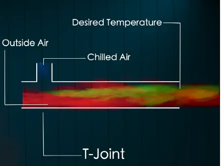
Fig. MixingTee

• As far as this challenge is considered , here we are taking two mixingTee i.e, one is short and other is long .In the X-direection ,the hot outside air is flowing and in vertical Y-direction, the cold air stream enters and results in mixing of same .In an accordance with that the desired temperature is obtained at the outlet.
• To study the effectiveness of mixing , a standard deviation plot graph is plotted in surface monitor at solution section of ansys fluent.
• In order to capture the turbulence and mixing ,we are taking the k-epsilon and k-omega turbulence model.
• Different momentum ratio is taken so that the outlet temperature variation is studied.
• k-epsilon is widely applied turbulence model base onpartial differential equations for the turbulent kinetic energy 'k' and its dissipation rate 'epsilon'.
• As far as turbulence is considered ,it is characterised by eddies with different space and time scales.Turbulence brings better mixing of a fluid and produces an additional diffusive effect. Such diffusion is known as eddy diffusion.
• At large Reynolds number there exists a continous transport of energy from large eddies to small eddies .Near the wall ,small eddies destroy themselves in dissipating energy i.e, converting kinetic energy of eddies into inter-molecular energy.
• In this problem , the fluid coming with high velocity(cold fluid) mixes with hot fluid ,the energy diffuses and mixing taking place and also momentum transfer due to velocity variation enables turbulence downstream of the mixing point.

PROCEDURE

• Geometry preparation : The geometry is being imported in spaceclaim and we have to extract the the wet volume , as we are interested in fluid flow and mixing .

• For this we have to prepare the geometry for extracting the fluid volume by selecting the edges of inletX , inletY and outlet respectively. Then we have to unselect the Shell1 for suppresing the physics so that the whole geometry is not going for meshing module.

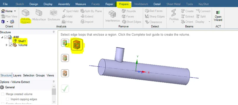
Fig. Geometry Preparation

MESHING

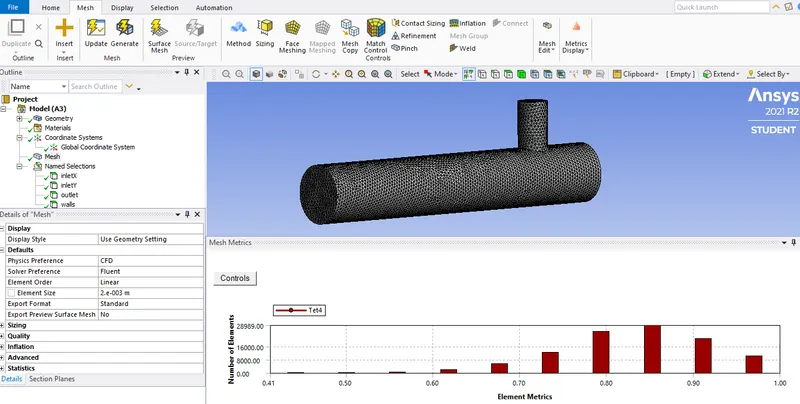
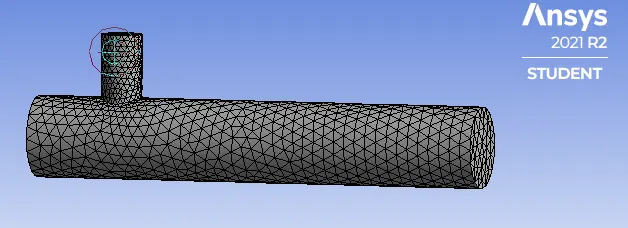
• In meshing module ,first we need to select the face and then name selection.
• In name selection we have to mention the inletX,inletYand outlet face respectively.
• First take the default mesh size element and then refine the mesh for further study.
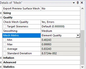
• Then we need to check Quality of meshand sure that it should be greater than 5%.Here the graph shows the minimum mesh quality is above 40%, which is acceptable.

SET UP

• In physics setup we have to select pressure based solver and absolute velocity formulation for steady state simulation.
• In pressure based approach ,the pressure field is extracted by solving a pressure or pressure correction equation which is obtained by manipulating continuity and momentum equation.

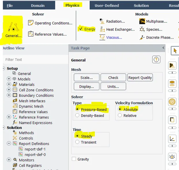
Fig. Physics setup

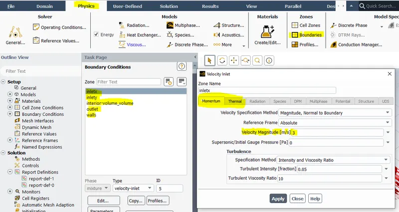
Fig. Boundary Condition set up

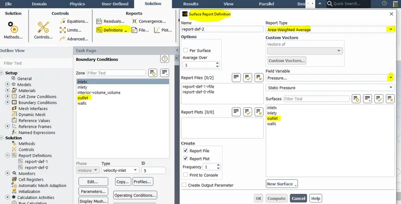
Fig. Solution setup

• In solution set up ,we have to study the outlet temperature of fluid mixing and to check the mixing effectiveness a standard deviation of outlet temperature should be checked out. For this data, we have to select defination in solution set up .

defination `rarr`new`rarr`surface report`rarr`report type`rarr`area weighted average`rarr`Field

variable`rarr`temperature`rarr`outlet

SET UP case for ShortTee (m=2) K-epsilon

• solver Type Pressure-based

• Velocity Formulation Absolute

• Time Steady

• viscous Model k-epsilon with standard wall function

• Material Air

• cell Zones Fluid type: air

• Boundaries inletX=velocity inlet in x-direction (Hot fluid)
  

velocity magnitude= 3 m/s

temperature magnitude= 36 deg C

inletY =velocity inlet in y-direction velocity magnitude=6 m/s

temperature magnitude = 19deg C

outlet= Pressure Outlet=Gauge Pressure=0 Pa

Walls- stationary wall

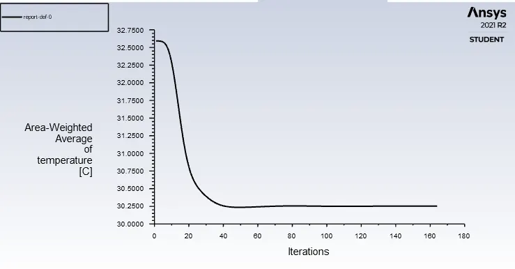
Fig.1 Area weighted Average of temperature Vs iterations for short Tee

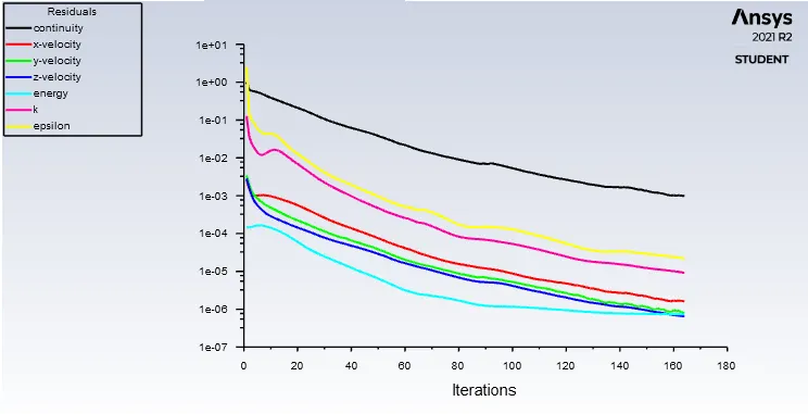
Fig.2 Residual Vs Iterations for Short Tee , momentum ratio =2

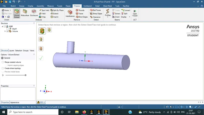
Fig.3 Volume extraction in Space claim

(a) (b)

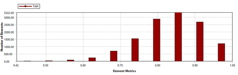
Fig.4 (a) meshing of shortTee,(b) Details of Mesh, (c) element metrics

(a) (b)

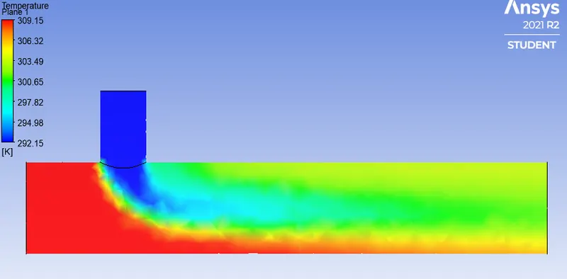
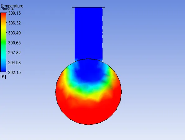
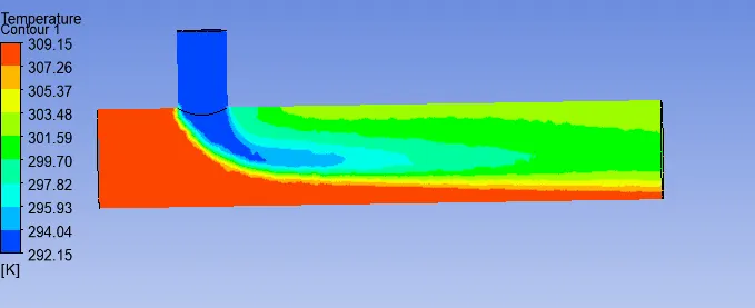
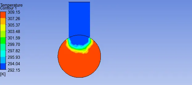
Fig.5 Plane showing variation of temperature (shortTee,m=2) (a) along the pipe (b) across the pipe

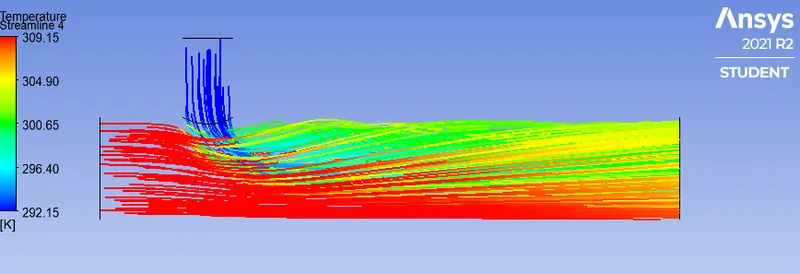
Fig.6 Temperature streamline along the pipe length (shortTee,m=2)

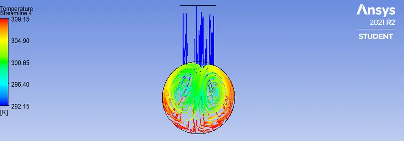
Fig.7 Temperature streamline across the pipe (shortTee,m=2)

(a) (b)

Fig.8 Temperature Contour (a) along the pipe length (shortTee,m=2) (b) across the pipe length

(a) (b)

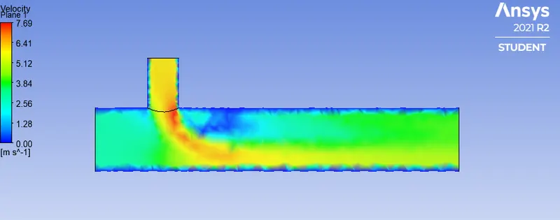
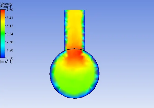
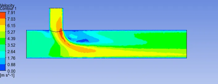
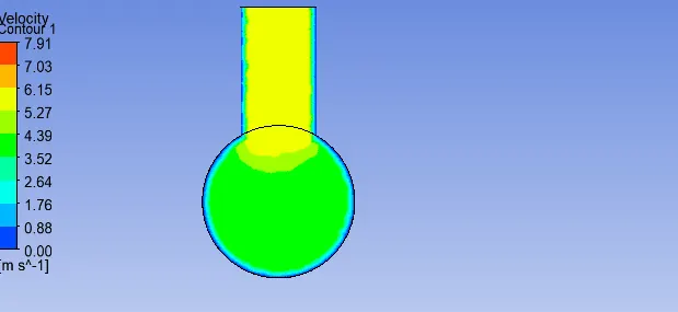
Fig.9 Plane showing velocity magnitude (a) along pipe length(b) across pipe length (shortTee,m=2)

(a) (b)

Fig.10 Velocity Contour showing (a) along pipe length(b) across pipe length (shortTee,m=2)

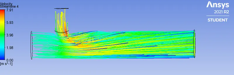
Fig.11 Velocity streamline along the pipe flow (shortTee,m=2)

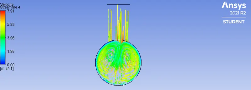
Fig.12 velocity streamline across the pipe length (shortTee,m=2)

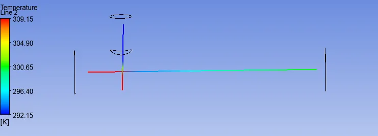
Fig.13 Temperature line plot along and across the pipe length (shortTee,m=2)

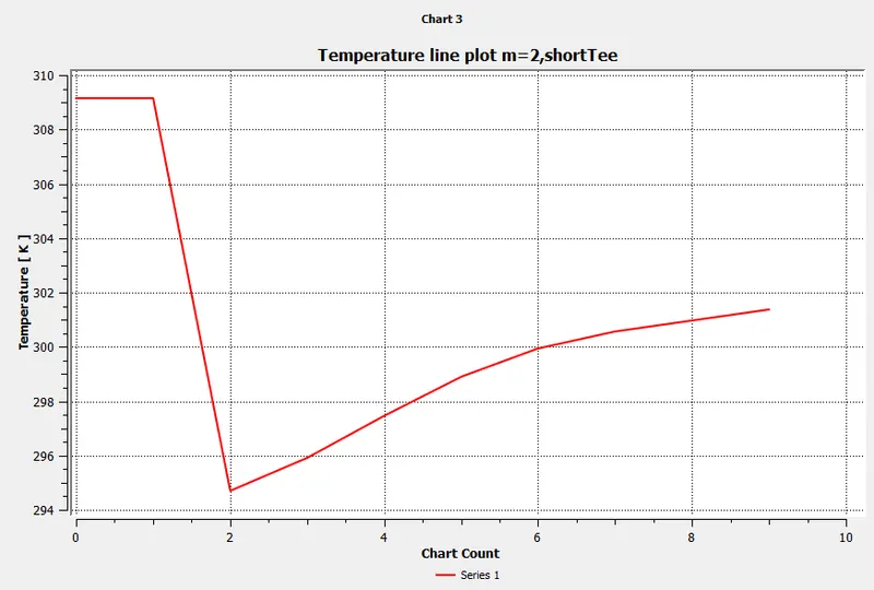
Fig.13 Graph plot from temperature line plot along pipe length (shortTee,m=2)

• This graph is plotted by taking the values from temperature line plot along the pipe length.This graph make sense as the temperature of mixing fluid decreases at the mixing point and then increases downstream of pipe.

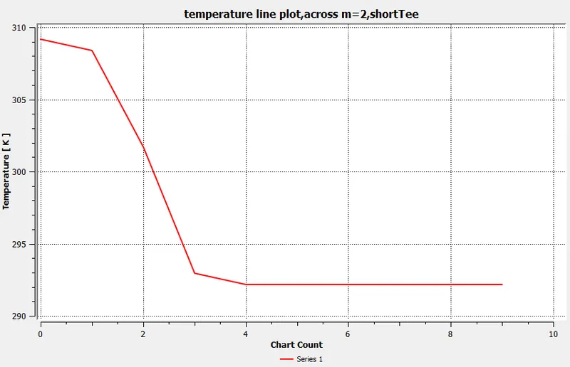
Fig.14 Graph plot from temperature line plot across pipe (shortTee,m=2)

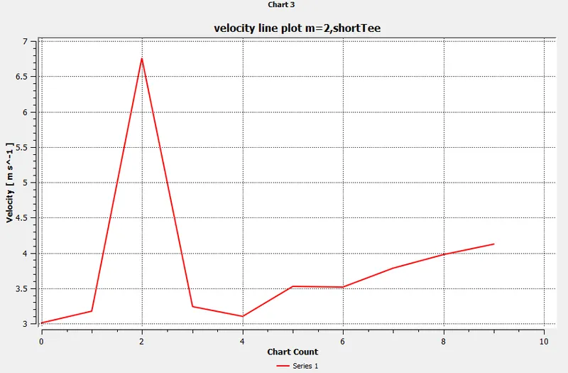
Fig.15 Graph plot from velocity line plot along pipe length (shortTee,m=2)

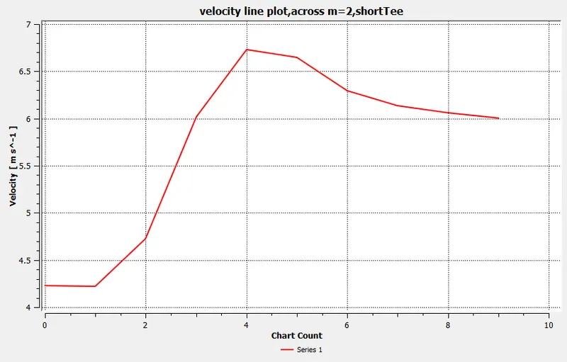
Fig.16 Graph plot from velocity line plot across pipe length (shortTee,m=2)

CASE 1.2 ShortTee, momentum Ratio=4

SET UP case for ShortTee (m=4) K-epsilon

• solver Type Pressure-based

• Velocity Formulation Absolute

• Time Steady

• viscous Model k-epsilon with standard wall function

• Material Air

• cell Zones Fluid type: air

• Boundaries inletX=velocity inlet in x-direction (Hot fluid)
  

velocity magnitude= 3 m/s

temperature magnitude= 36 deg C

inletY =velocity inlet in y-direction velocity magnitude=12 m/s

temperature magnitude = 19deg C

outlet= Pressure Outlet=Gauge Pressure=0 Pa

Walls- stationary wall

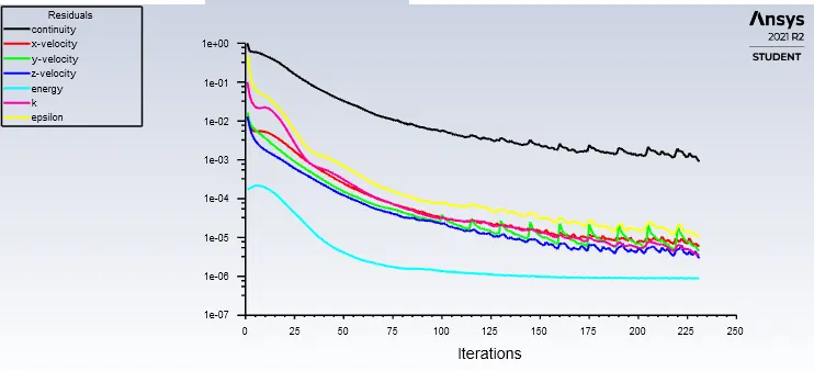
Fig.17 Residual Vs Iterations for Short Tee , momentum ratio =4

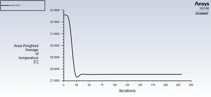
Fig.18 Area weighted Average of temperature Vs iterations for short Tee (m=4)

Fig.19 Volume extraction of fluid volume in Space claim

Fig.20 Meshing

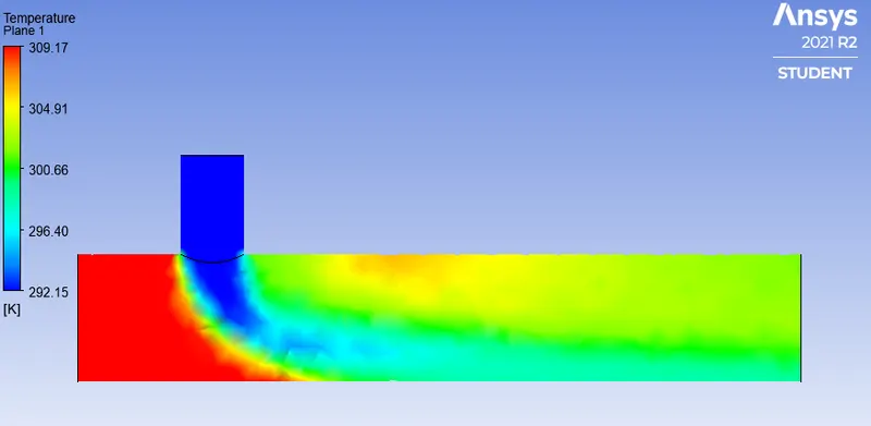
(a) (b)

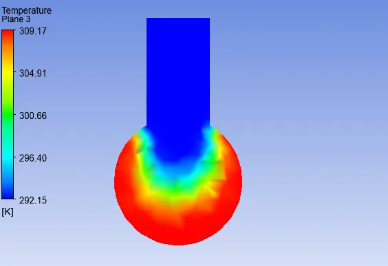
Fig.21 Plane showing Temperature magnitude (a) along the pipe length (b) across pipe length

(a) (b)

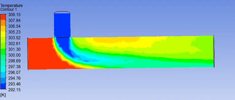
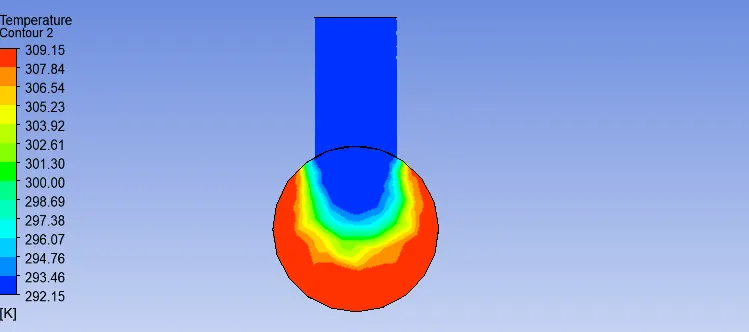
Fig.22 Contour showing Temperature magnitude (a) along the pipe length (b) across pipe length( shortTee,m=4)

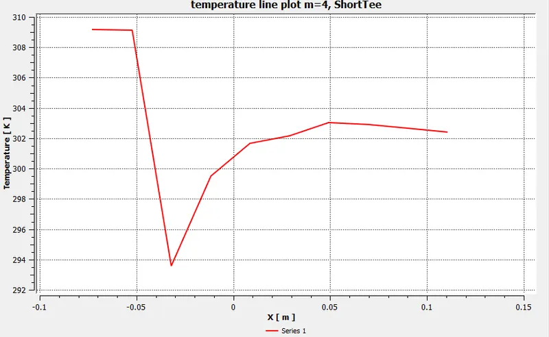
Fig.23 Graph plot from temperature line plot along pipe length (shortTee,m=4)

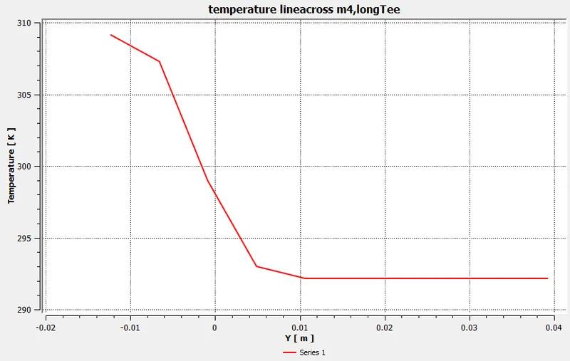
Fig.24 Graph plot from temperature line plot across pipe length (shortTee,m=4) , line taken at the

mid-section of inlet Y

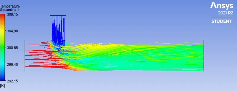
Fig.25 Temperature streamline along the pipe length (shortTee,m=4)

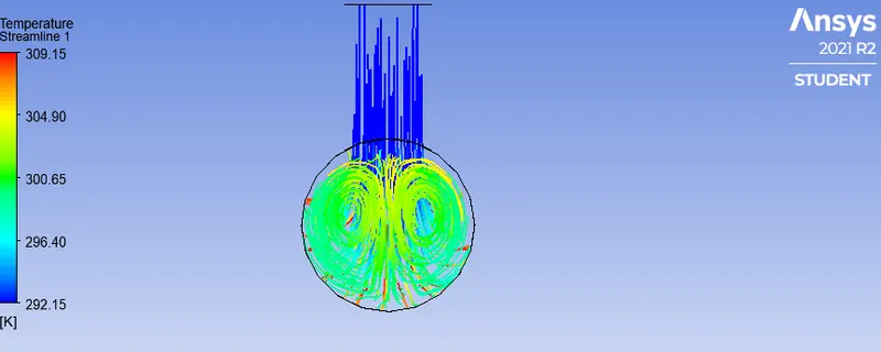
Fig.26 Temperature streamline across the pipe length (shortTee,m=4)

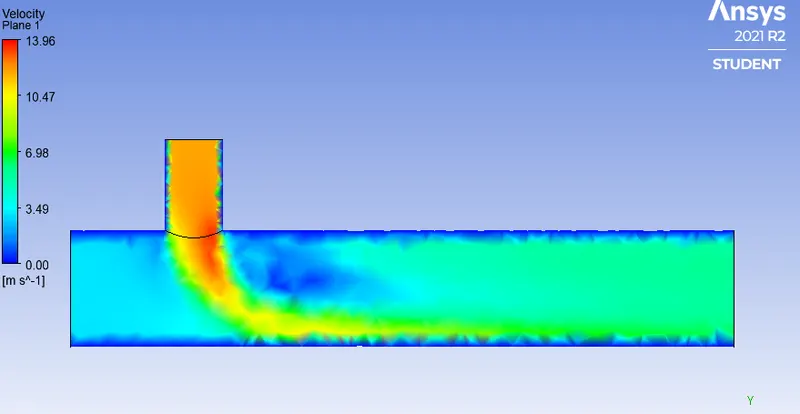
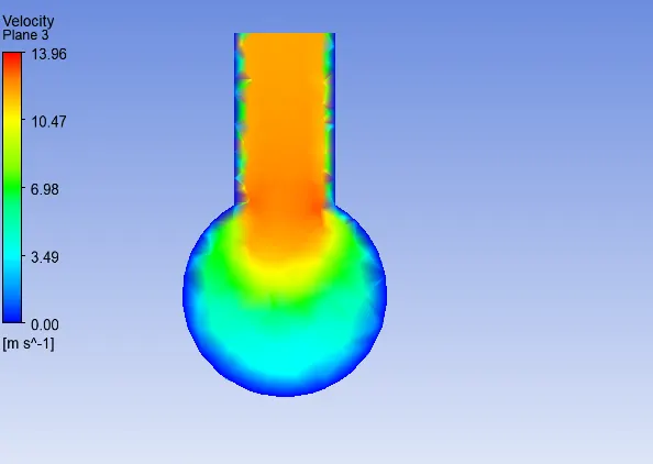
(a) (b)

Fig.27 Plane showing velocity magnitude (a) aong pipe length (b) across pipe

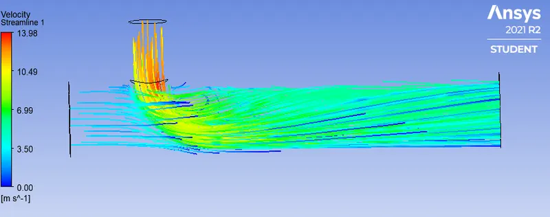
Fig.28 Velocity streamline along pipe length (m=4)

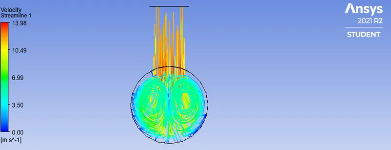
Fig.29 velocity streamline across pipe (m=4)

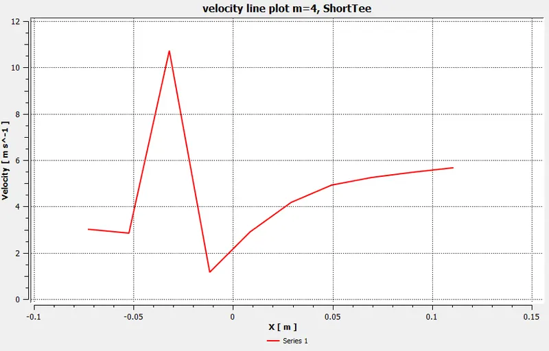
Fig.30 Graph plotted from velocity line plot along pipe (shortTee,m=4)

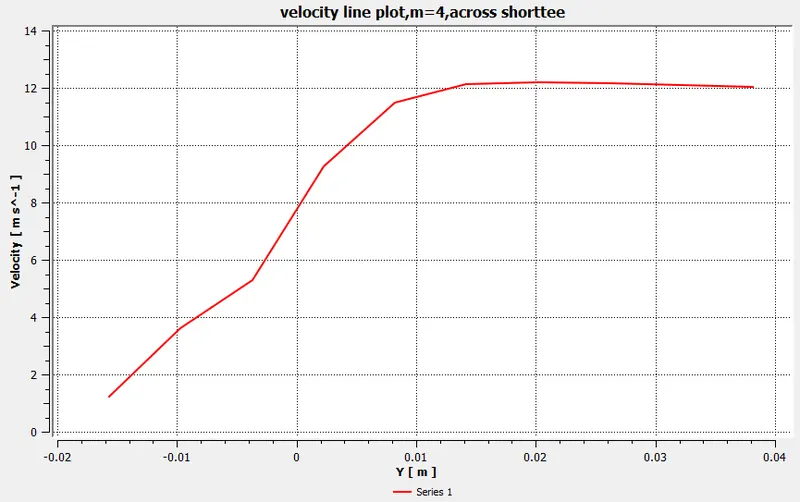
Fig.31 Graph plotted from velocity line plot across pipe (shortTee,m=4)

CASE 2.1 Long Tee, Momentum ratio=2

SET UP case for LongTee (m=2) K-epsilon

• solver Type Pressure-based

• Velocity Formulation Absolute

• Time Steady

• viscous Model k-epsilon with standard wall function

• Material Air

• cell Zones Fluid type: air

• Boundaries inletX=velocity inlet in x-direction (Hot Fluid)
  

velocity magnitude= 3 m/s

temperature magnitude= 36 deg C

inletY =velocity inlet in y-direction (Cold Fluid) velocity magnitude=6 m/s

temperature magnitude = 19deg C

outlet= Pressure Outlet=Gauge Pressure=0 Pa

Walls- stationary wall

PLOTS

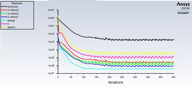
Fig.32 Residual Vs Iterations for Long Tee , momentum ratio =2

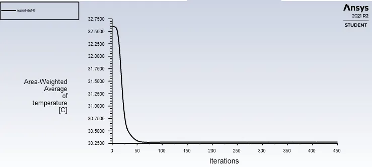
Fig.33 Area weighted Average of temperature Vs iterations for LongTee (m=2)

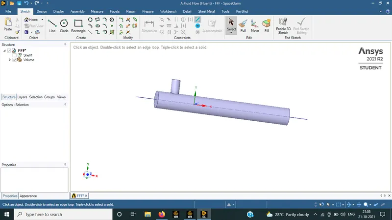
Fig.34 Geometry preparation

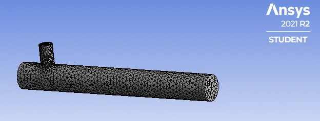
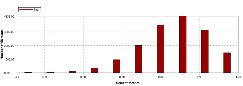
Fig.35

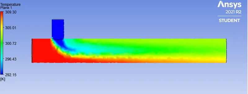
Fig.36 plane showing Temperature magnitude along pipe length( longTee,m=2)

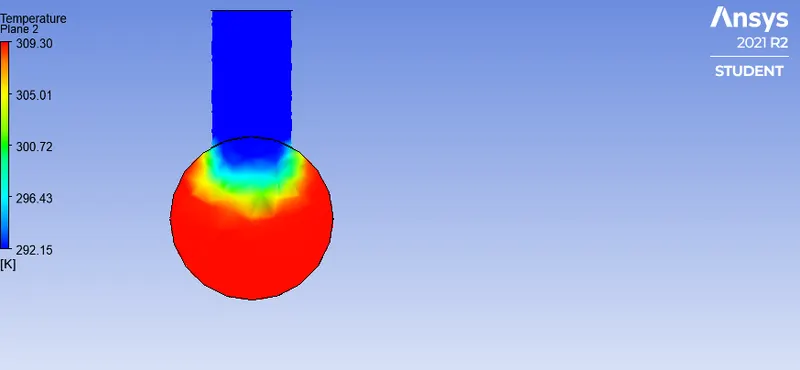
Fig.37 plane showing Temperature magnitude across pipe length( longTee,m=2)

(a) (b)

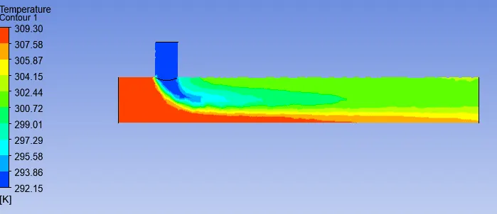
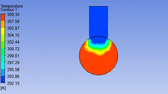
Fig.38 contour showing Temperature magnitude (a) along pipe length (b) across pipe ( longTee,m=2)

(a) (b)

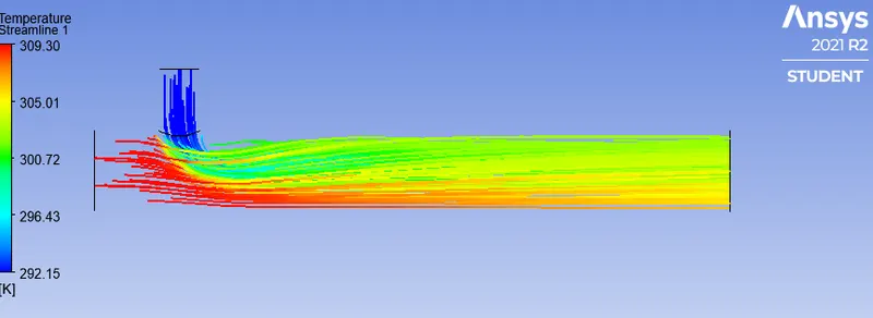
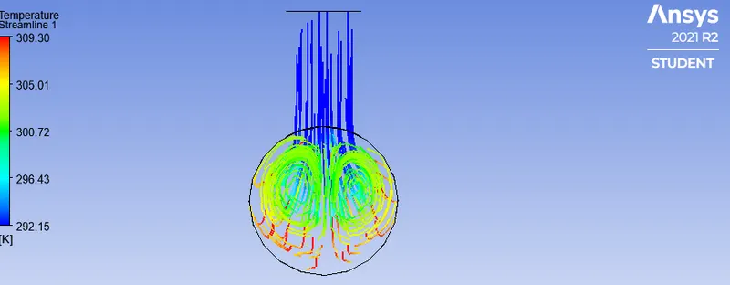
Fig.39 Temperature streamline (a) along pipe length (b) across pipe length (longTee,m=2)

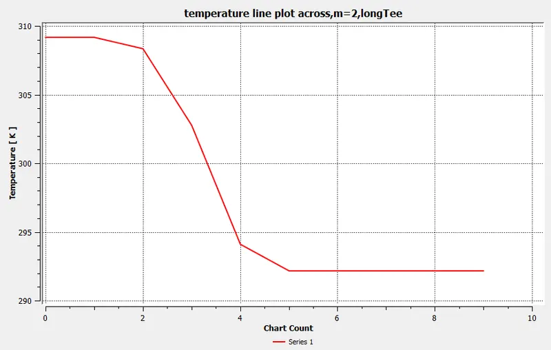
Fig.40 Graph plotted from temperature line plot across pipe (longTee,m=2)

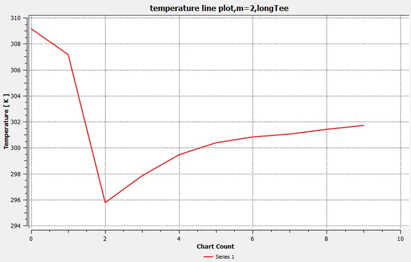
Fig.41 Graph plotted from temperature line plot along the pipe length (longTee,m=2)

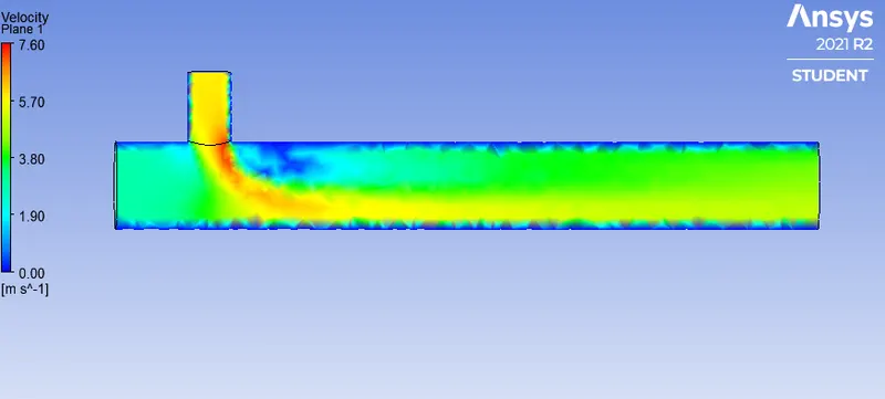
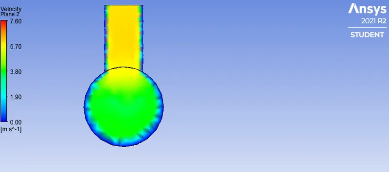
(a) (b)

Fig.42 Plane showing velocity magnitude (a) along pipe length (b) across pipe (longTee,m=2)

(a) (b)

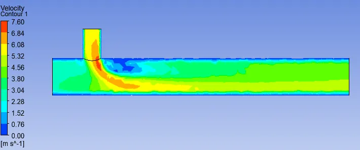
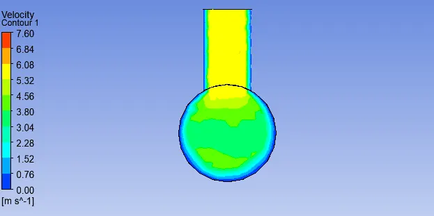
Fig.43 Contour showing velocity magnitude (a) along pipe length (b) across pipe ( longTee, m=2)

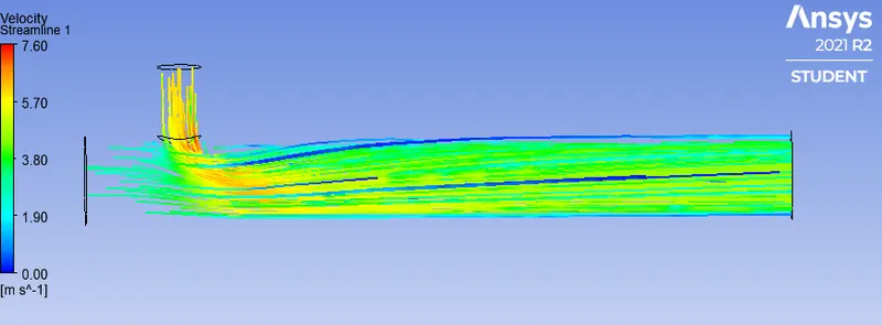
Fig.44 Velocity streamline velocity magnitude along pipe length ( longTee, m=2)

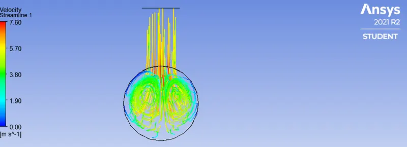
Fig.45 Velocity streamline velocity magnitude across pipe ( longTee, m=2)

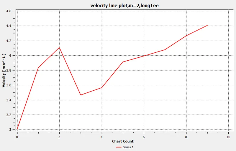
Fig.46 graph plotted from velocity line plot along pipe length (longTee,m=2)

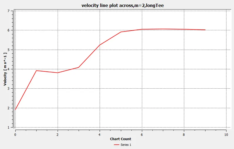
Fig.47 graph plotted from velocity line plot across pipe length (longTee,m=2)

CASE 2.2

• LongTee, m=4, Having inlet cold fluid velocity= 12 (m/s)

SET UP case for LongTee (m=4) K-epsilon

• solver Type Pressure-based

• Velocity Formulation Absolute

• Time Steady

• viscous Model k-epsilon with standard wall function

• Material Air

• cell Zones Fluid type: air

• Boundaries inletX=velocity inlet in x-direction (Hot Fluid)
  

velocity magnitude= 3 m/s

temperature magnitude= 36 deg C

inletY =velocity inlet in y-direction (Cold Fluid) velocity magnitude=12 m/s

temperature magnitude = 19deg C

outlet= Pressure Outlet=Gauge Pressure=0 Pa

Walls- stationary wall

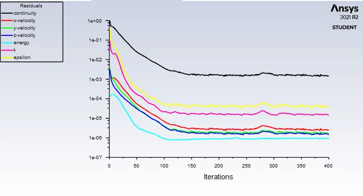
Fig.48 Residual Vs Iterations ( Long Tee , momentum ratio =4)

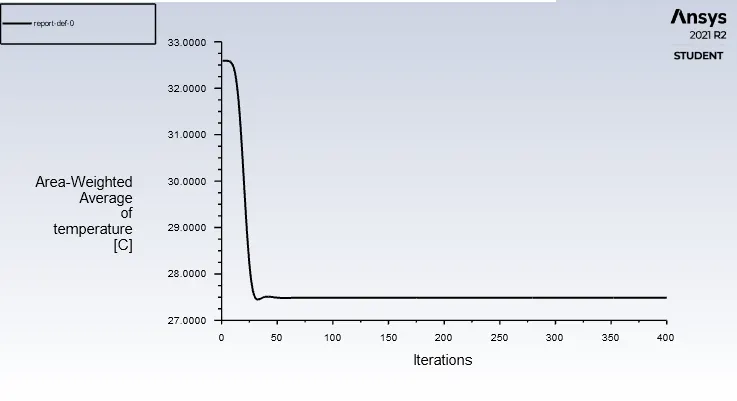
Fig.46 Area weighted Average of temperature Vs iterations for LongTee (m=4)

Fig.47 Geomety preparation

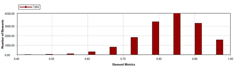
Fig.48 meshing and element metrices

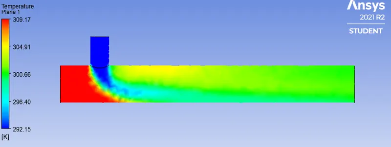
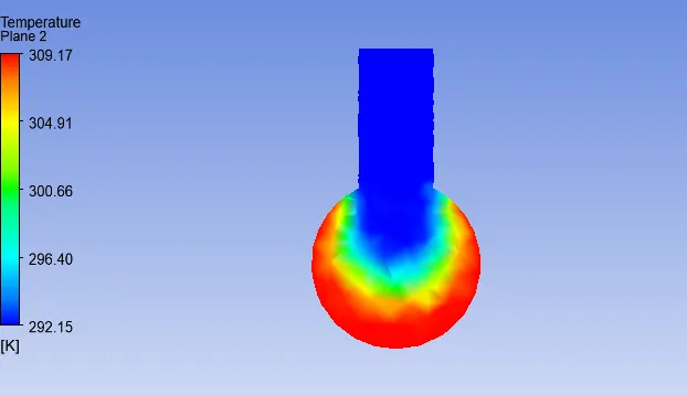
(a) (b)

Fig.49 plane showing temperature magnitude (a) along pipe length (b) across pipe (LongTee,m=4)

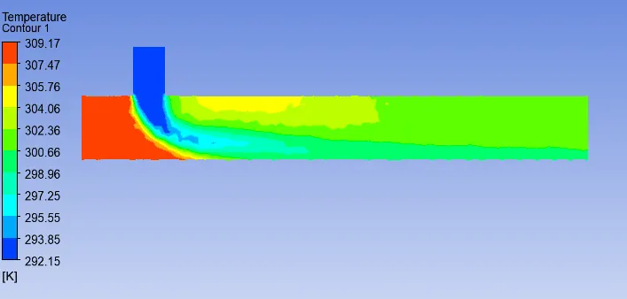
(a) (b)

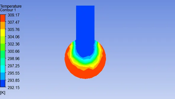
Fig.50 Contour showing temperature magnitude (a) along pipe length (b) across pipe (LongTee,m=4)

(a) (b)

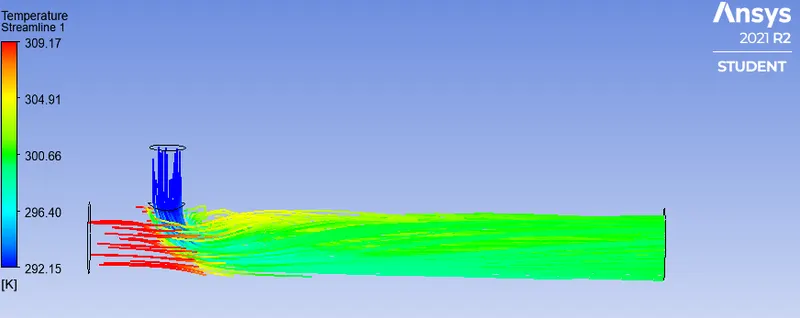
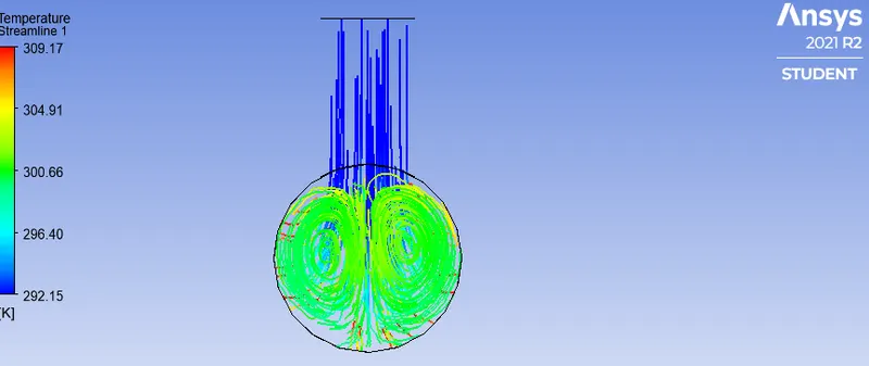
Fig.51 temperature streamline (a) along pipe length (b) across pipe (LongTee,m=4)

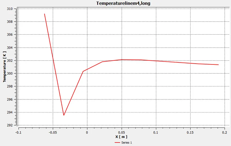
Fig.52 Graph plotted from temperature line plot along pipe length (longTee,m=4)

Fig.53 Graph plotted from temperature line plot across pipe (longTee,m=4)

(a) (b)

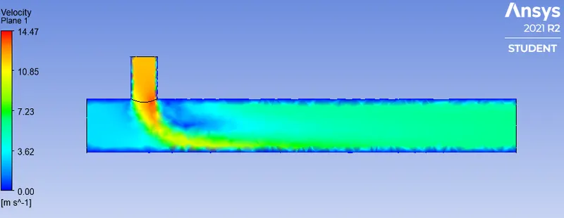
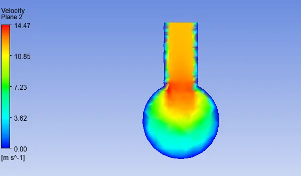
Fig.54 Plane showing Velocity magnitude (a) along pipe length (b) across pipe (LongTee,m=4)

(a) (b)

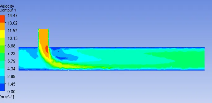
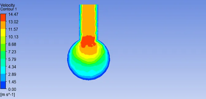
Fig.56 Contour showing Velocity magnitude (a) along pipe length (b) across pipe (LongTee,m=4)

(a) (b)

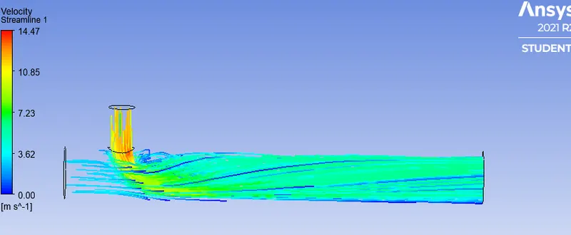
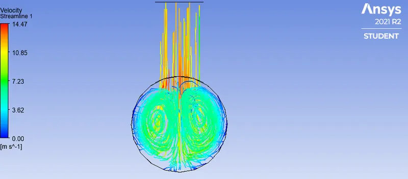
Fig.57 velocity streamline showing (a) along pipe length (b) across pipe (LongTee,m=4)

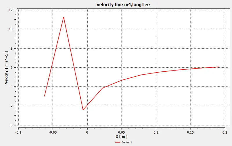
Fig.58 Graph plotted from Velocity line plot along pipe (longTee,m=4)

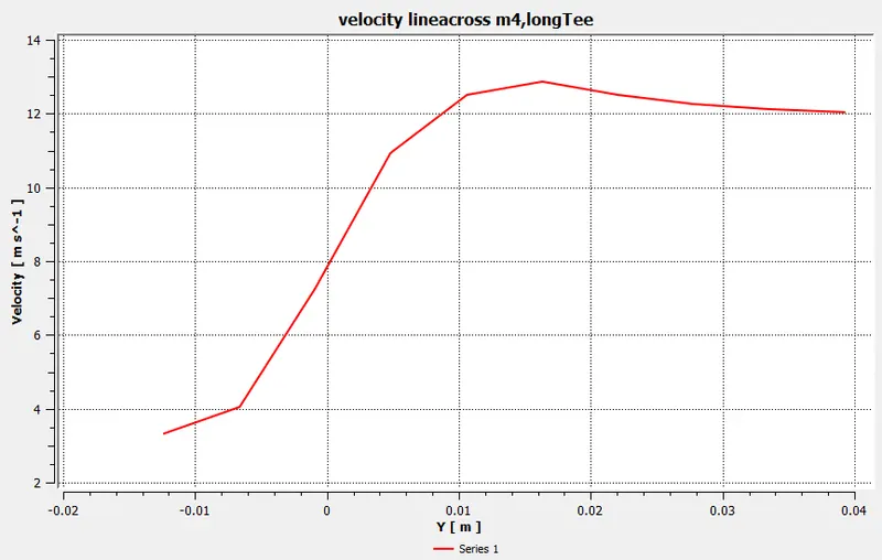
Fig.59 Graph plotted from Velocity line plot across pipe (longTee,m=4)

ShortTee, m=2 and m=4, k-Omega

SET UP case for ShortTee (m=4) K-omega

• solver Type Pressure-based

• Velocity Formulation Absolute

• Time Steady

• viscous Model k-omega SST Model

• Material Air

• cell Zones Fluid type: air

• Boundaries inletX=velocity inlet in x-direction (Hot Fluid)
  

velocity magnitude= 3 m/s

temperature magnitude= 36 deg C

inletY =velocity inlet in y-direction (Cold Fluid) velocity magnitude=6 m/s

temperature magnitude = 19deg C

outlet= Pressure Outlet=Gauge Pressure=0 Pa

Walls- stationary wall

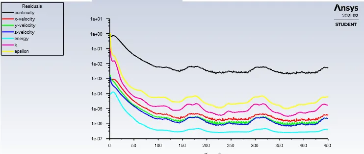
Fig.60 Residual Vs Iterations ( shortTee , momentum ratio =2)

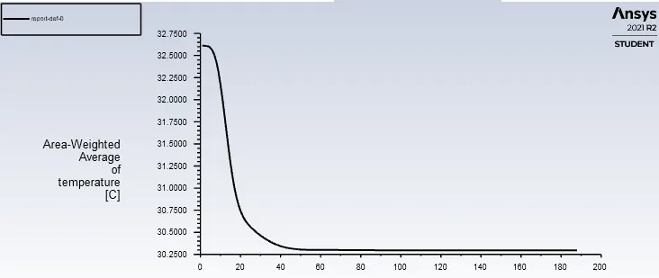
Fig.61 Area weighted Average of temperature Vs iterations for ShortTee (m=2)

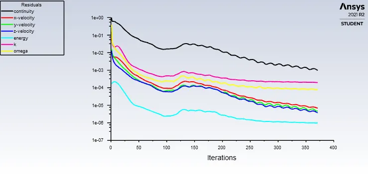
Fig.62 Residual Vs Iterations ( shortTee , momentum ratio =4)

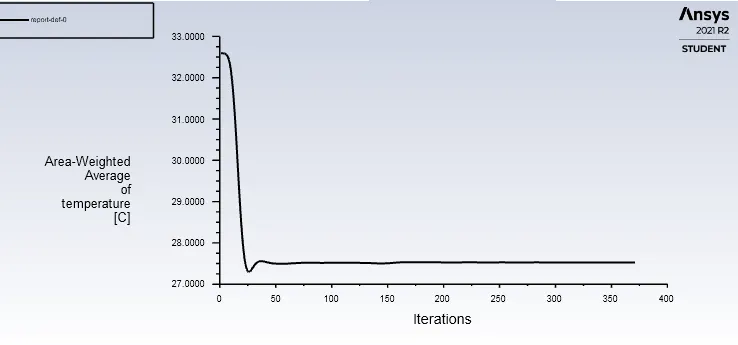
Fig.63 Area weighted Average of temperature Vs iterations for ShortTee (m=4)

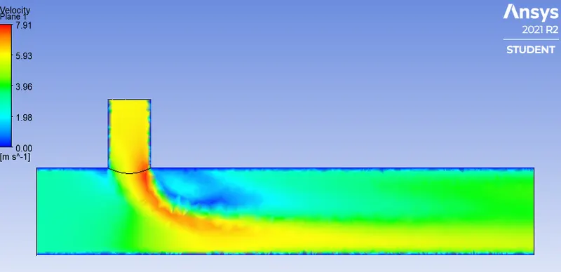
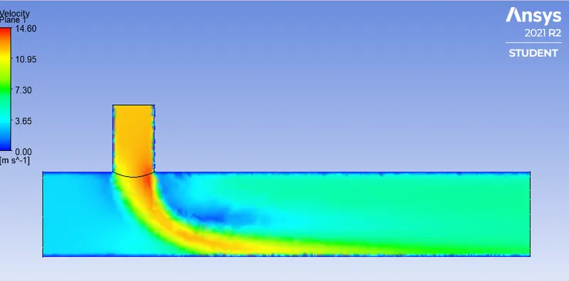
(a) (b)

Fig.64 Plane showing Velocity magnitude (a) for m=2, shortTee (b) for m=4,shortTee

ShortTee

m=2 m=4

cell size 0.01 0.01

avg. outlet temperature 30.295 27.527

standard deviation 1.249 1.130

number of iteration 250 300-350

Turbulence model k-Omega k-omega

shortTee LongTee

m=2 m=4 m=2 m=4

Average outlet temperature 30.253 27.566 30.276 27.487

Standard deviation 2.315 1.261 1.487 0.5148

Cell count 12546 12546 15566 15566

Mesh size 0.01 0.01 0.01 0.01

Number of iteration 163 231 250 250

Turbulence Model K-epsilon K-epsilon k-epsilon k-epsilon

• Grid independent test : Here the mesh size is taken as 0.002 m or 2mm

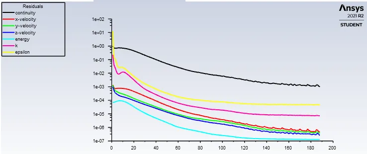
Fig.65 Residual Vs Iterations ( shortTee , momentum ratio =2)

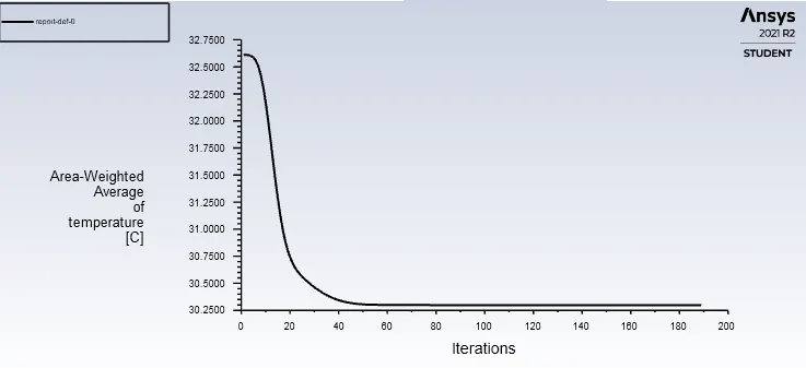
Fig.66 Area weighted Average of temperature Vs iterations (ShortTee, m=2)

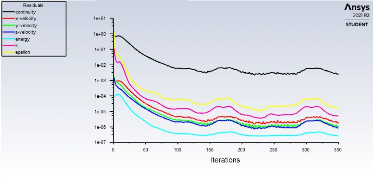
Fig.67 Residual Vs Iterations ( shortTee , momentum ratio =4)

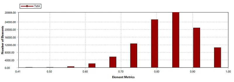
Fig.68

shortTee

m=2 m=4

Average outlet temp. 30.297 27.588

Number of iteration 192 250-300

Standard deviation 2.315 1.322

cell count 105295 105295

• As the size of mesh element is refined to 0.002m from 0.01m , the outlet temperature remains same irrespective of the momentum ratio(velocity of inletX/velocity of inletY).
• The number of iteration increases for momentum ratio 4, as the mixing taking place with high velocity ,momentum transfer enables the calculation to be much more time consuming and convergence criterion is reached with more number of iteration.

Analytical Result

`T_(mixture)=(dotm_(hot)*T_(hot)+dotm_(cold)*T_(cold))/(dotm_(hot)+dotm_(cold))`

• In order to calculate the mixture temperature ,we need to calculate the mass of hot and cold fluid respectively.

As we know mass=density * volume

`dotm=rho_(air)*A_(cross-section)*Velocity`

mass of Hot fluid= density of air * area of cross-section * velocity of hot fluid

density of air= 1.225 kg/m^3

velocity of hot fluid = 3 (m/s) area of cross-section of inletX=`0.901 *10^(-3)`

velocity of cold fluid = 6 (m/s) area of cross-section of inletY =`0.225*10^(-3)`

• mass flow rate of hot fluid= 1.225*3*0.901*10^(-3)=3.31 (g/s) m=2
• mass flow rate of cold fluid= 1.225*6*0.225*10^(-3)=1.65 (g/s) m=2

simulation results for mass flow rate

• mass flow rate of hot fluid = 3.32 (g/s) m=2
• mass flow rate of cold fluid= 1.63 (g/s) m=2

• temperature of mixture = `T_(mixture)=(dotm_(hot)*T_(hot)+dotm_(cold)*T_(cold))/(dotm_(hot)+dotm_(cold))`

= 303.3 K m=2

• temperature of mixture =`T_(mixture)=(dotm_(hot)*T_(hot)+dotm_(cold)*T_(cold))/(dotm_(hot)+dotm_(cold))`

= 300.5 k m=4

• So it is validated from simulation result that the outlet temperature of mixture in both cases are 30.253 deg C and 27.588 deg C, therefore it is making sense with the analytical results.

Conclusion

• If we consider length of pipe, the longTee with momentum ratio 4 is giving more mixing effectiveness as compared to shortTee.It is cleared from the standard deviation graph that the outlet temperature for m=4, is lower than m=2 for both cases.
• The outlet temperature for short and longTee at m=2 is same ,though SD is different.SD is more in shortTee due to temperature gradient and improper mixing of fluid stream.
• SD for long tee at m=4 is lower than shortTee at m=4. In both cases the momentum ratio remains same but length of pipe plays an important factor that enables the proper mixing and energy cascading i.e, the eddies generated at the mixing point are dissipated to the adjacent fluid particles by diffusion and advection .
• K-epsilon model converges faster as compared to k-omega turbulence model. k-omega model is best suited for flow separation,flow near walls and for adverse pressure gradient as in the case of flow through nozzle in I.C engines. So for fluid mixing and pipe flow ,we are interested for the desired outlet temperature and not for thermal gradient near walls (thermal stripping), k-epsilon model s taken for consideration.