Week 1: Channel flow simulation using CONVERGE CFD
Aim
To simulate airflow through the given rectangular channel geometry using Converge CFD and analyze the results using various mesh sizes.
Introduction
A simple airflow simulation is conducted on the rectangular 2D channel geometry shown below.
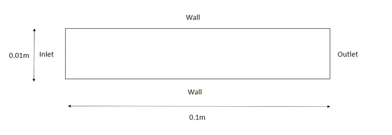
Method
Mesh Generation
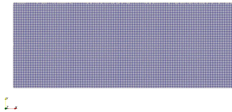
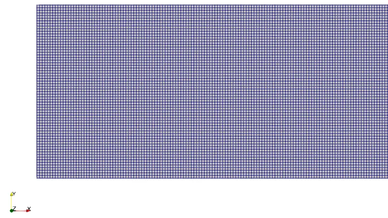
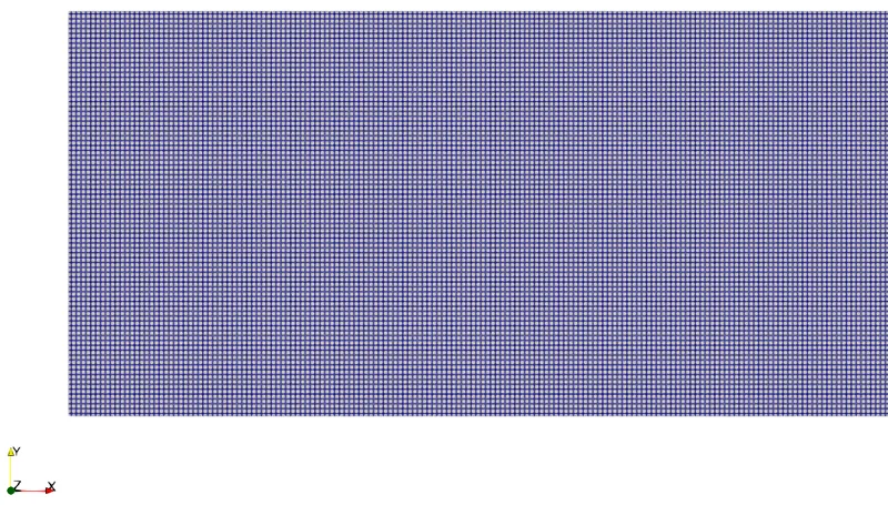
A uniform structured grid was generated over the geometry. A total of three meshes were generated to observe the changes in the results due to mesh. The element sizings for the three meshes were set to 2e-4m, 1.5e-4m, and 1.2e-4m. The results of the mesh generation can be seen in the images below.
Mesh1 - 25k cells
Mesh 2 - 45k cells
Mesh 3 - 70k cells
CFD Setup
All Simulations were conducted using Converge v3.0. The fluid used in the domain was air with default properties. The pressure at the inlet was set to 100001Pa and the pressure outlet was set to 100000Pa. The top and bottom walls of the channel were set to no-slip condition. The front and back faces of the domain were given the TwoD boundary condition which acts as a form of symmetry.
The steady-state density-based PISO solver was used for the spatial discretization of the flow parameters. Momentum, density, energy, and species were estimated using the SOR scheme while pressure was estimated using the converge bicgstab scheme. Turbulence in the flow was assumed to be negligible.
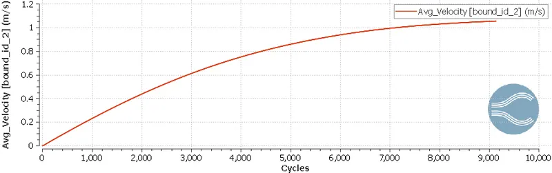
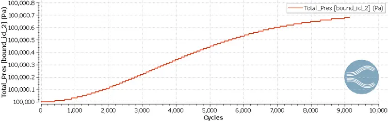
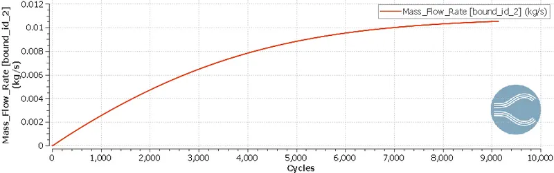
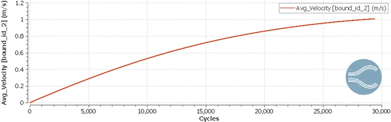
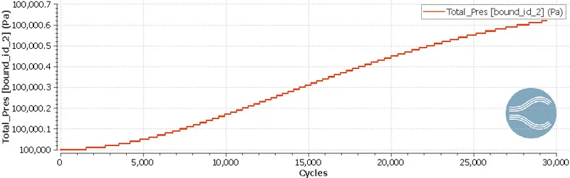
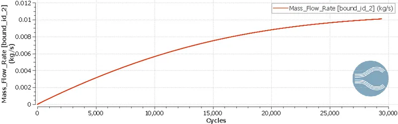
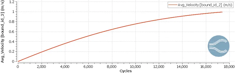
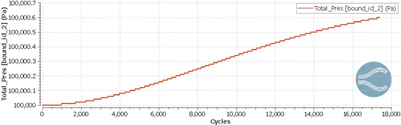
Convergence was monitored using monitors of average velocity, pressure, and mass flow rate at the outlet. The solution was deemed converge when the monitors varied under 0.001 units across iterations.
Results
The images below show the monitors of velocity, pressure, and mass flow rate at the outlet to ensure convergence of Mesh 1
The images below show the monitors of velocity, pressure, and mass flow rate at the outlet to ensure convergence of Mesh 2.
The images below show the monitors of velocity, pressure, and mass flow rate at the outlet to ensure convergence of Mesh 3.
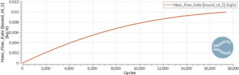
The images below show the comparison of the velocity profile at the outlet for the various meshes.
Mesh 1
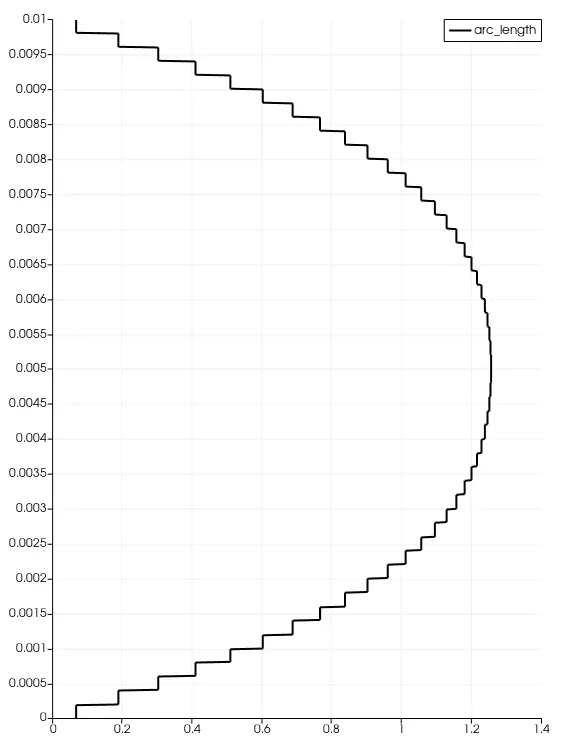
Mesh 2
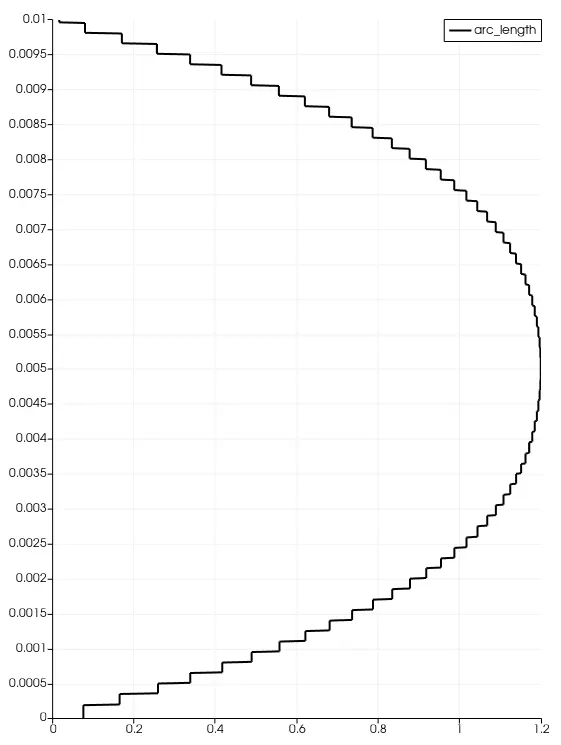
Mesh 3
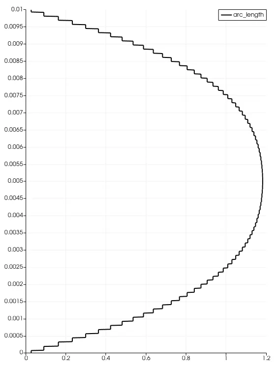
From the velocity profiles, it can be seen that there is an increased velocity prediction in Mesh 1. Upon mesh refinement the peak velocity can be seen to reduce.
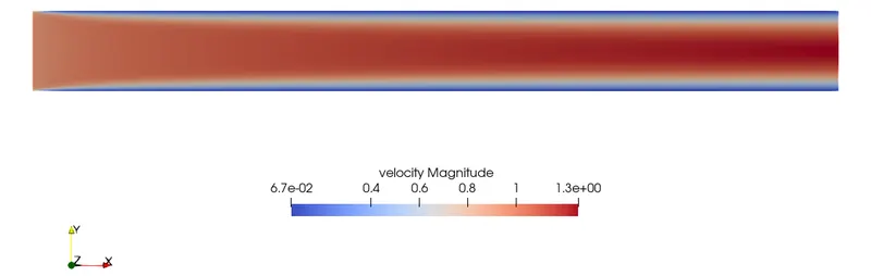
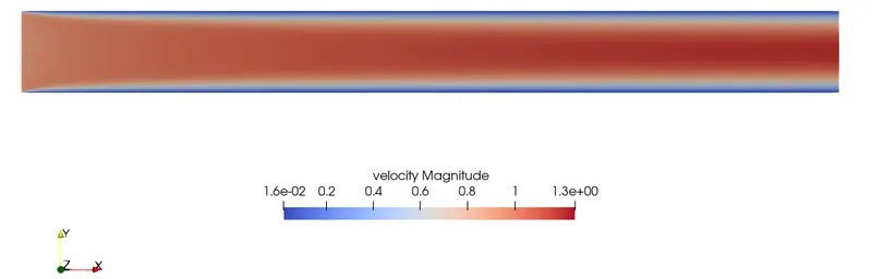
The images below show the comparison of the velocity contour for the various meshes.
Mesh 1
Mesh 2
Mesh 3
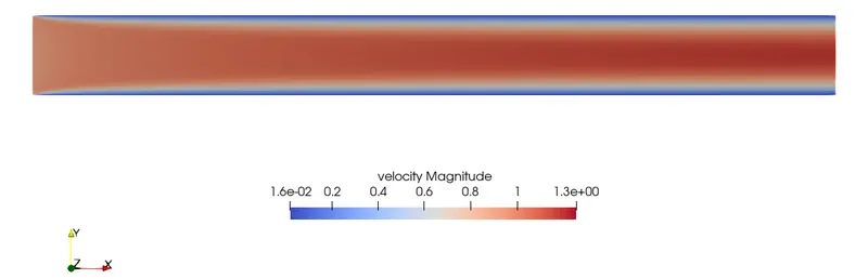
The velocity contours are seen to be similar for all the cases with better resolution of the boundary layer seen in the refined mesh cases.
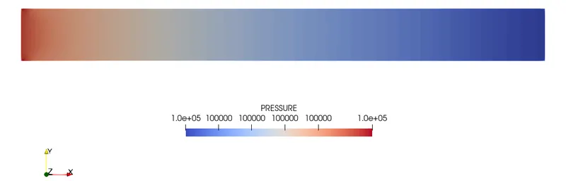
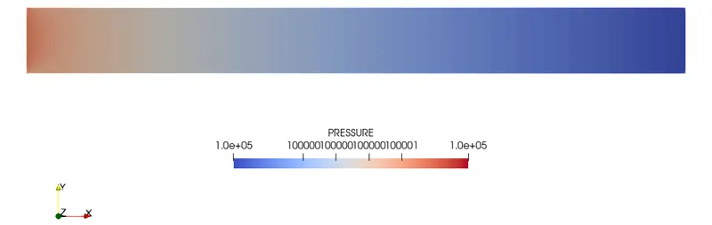
The images below show the comparison of the pressure contour for the various meshes.
Mesh 1
Mesh 2
Mesh 3
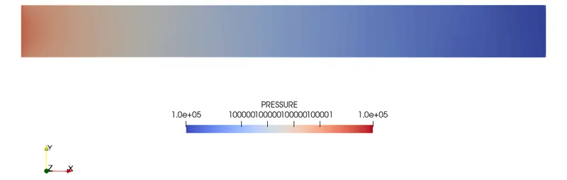
The pressure contours do not show any significant difference with change in mesh since the pressure difference across the inlet and the outlet is very small.
An animation of the flow development by the solver across iterations is attached to the link below:
https://drive.google.com/file/d/1ttOE_SZggYF2oNsiAu85U7FpgPOyU_IU/view?usp=sharing
The animation shows the initialization of the flow using the boundary conditions and the pressure difference between the inlet and outlet slowly driving the airflow until a steady state is achieved.
Conclusion
Simulations of airflow over the given rectangular channel were conducted using converge. The analysis was conducted over three meshes of varying densities. It was seen that the coarse mesh predicted a higher velocity at the outlet compared to the refined mesh cases. Further, it was seen that the refined mesh cases had a better resolution of the boundary layer flow.