Week 1: Channel flow simulation using CONVERGE CFD

Aim:
To simulate flow of air through a square duct in converge.
Introduction:
The flow is induced in the square duct of 0.1 m length with a pressure difference of 1 Pa. Given the minor change in pressure, the velocity and hence reynolds number would also be insignificant. A laminar flow assumption is valid for this case. Also, since the flow cross-section is uniform, the flow will reach steady state eventually after the flow starts at inlet. Hence steady state simulation would be sufficient to analyse the end results. The case will be solved with three different meshes to analyse the effect of cell size on results.
Case setup in Converge:
1. Open converge studio and create a box of size 0.1*0.01*0.01 m using the box option under Create->Shape

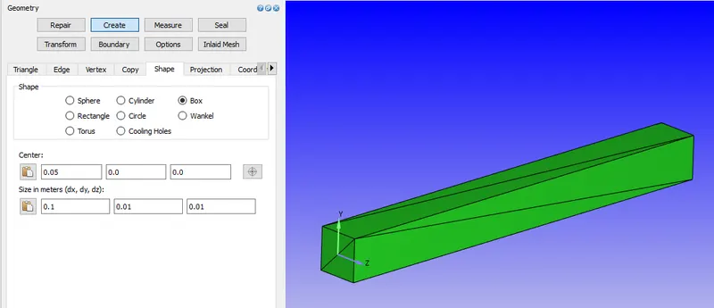
2. Enable normals view on graphics toolbar. Invert the normal so that the normals point towards the fluid material point using "propagate change from single triangle" option from Transform->Normal tab

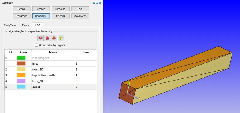
3.Create boundaries from geometry faces using Boundary-> flag tab. Create 5 boundaries using "create multiple boundaries option". Rename the boundaries to meaningful names such as inlet, outlet, wall, etc as shown. Assign the faces on -X to inlet; +X to outlet, -Z and +Z to 2D boundaries, -Y and +Y to walls.
image

4.Click on begin case setup from right tree. Set application type to "Time-based". In Materials tab, set material to predefined mixture "air", disable "reaction mechanism" and enable "species". In physical models tab, disable "Turbulence modelling" and apply. The case setup tree shows up
5. Open species tab, add O2 and N2 to the gas species list
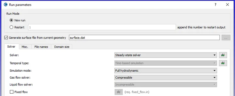
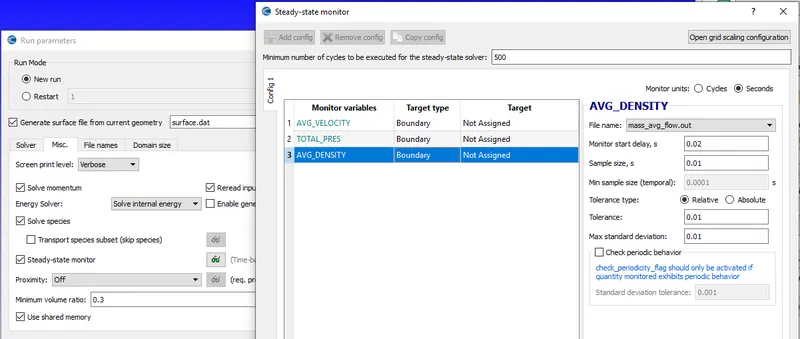
6. Under run parameters, set solver to "steady-state". Under Misc tab, enable steady-state monitor and set the monitor vars to avg_velocity, total_pres and avg_density at boundaries.

7. Under simulation time parameters, set start time to 0 and end time to 15000 cycles. Set intial and minimum time-step to 1e-9 and max time-step to 1
8. In solver parameters, under equations, set preconditioner of pressure to none
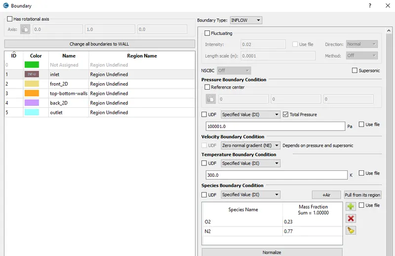
9. Open boundaries, set inlet type to inflow with total pressure of 1,00,001 Pa; temperature to 300 K; and species mass fraction to O2 - 0.23 and N2 - 0.77. Set front and back boundaries as two_D; top-bottom-walls as no-slip walls with zero gradient for temperature. Outlet bc is set as outflow boundary condition with static pressure 1,00,000 Pa. Backflow temperature and species are set similar to inflow bc

10. Under regions and initialization, a new region "region 0" is created. It's set to be initiazed with velocity of 0 m/s, temperature of 300 K and pressure of 1 atm. Intial species mass fraction is set as O2 - 0.77 and N2 - 0.23. Incorrect species mass fraction is set delibrately to show that intial condition doesn't determine the steady state solution for most cases.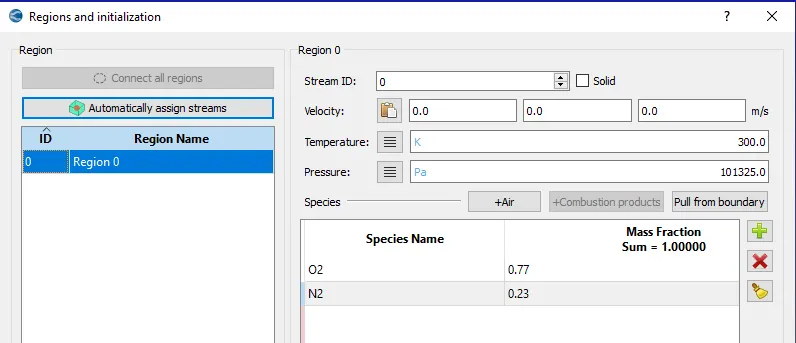

11. Open boundary conditions and assign "region 0" to all the boundaries created
12. Open steady-state monitors and set all monitors to outlet
13. Open base grid and dx, dy and dz to 2e-4 for case1.
14. Open post variable selection and disable turbulence quantities from Combustion/Turbulence tab. Add mass fraction of O2 and N2 from species tab.
15 Open output files, set time-interval for 3D output data and writing restart files to 100 cycles. Set max number of restart files to 3.
16. Export all input files to a run folder created for case1. Run the converge solver in run folder using cygwin.
17. Similar set dx, dy and dz to 1.5e-4 and 1.2e-4 for cases 2 and 3. Run converge solver for all the cases.
18. In post-processing window of converge, convert all the post files with all variables to paraview binary format and open the vtk files in paraview to post-process.
Results:
case1:

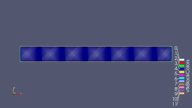
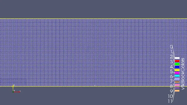
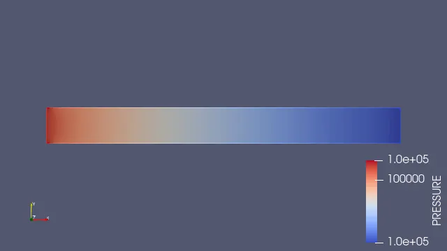
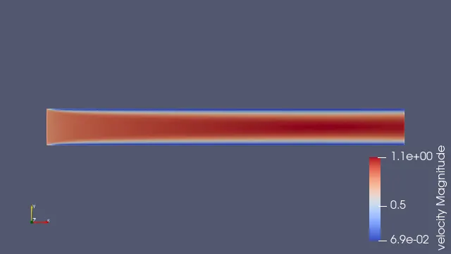
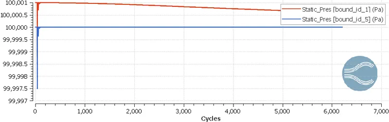
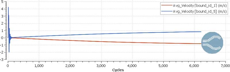
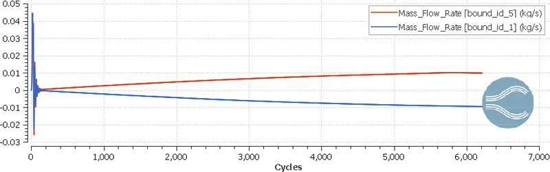
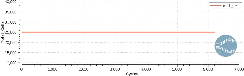
case2:

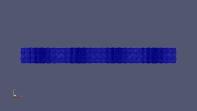
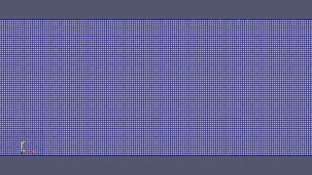
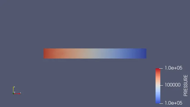
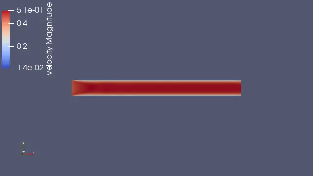
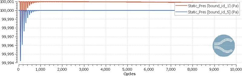
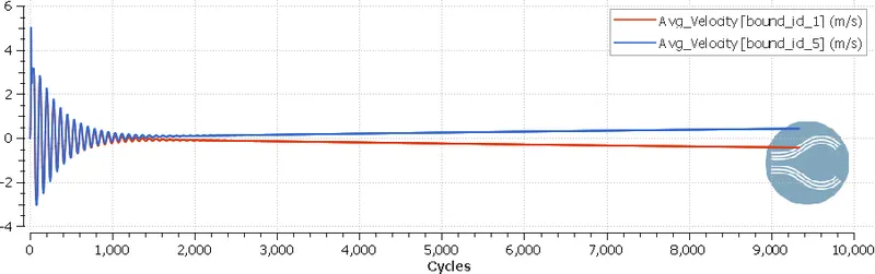
case3:

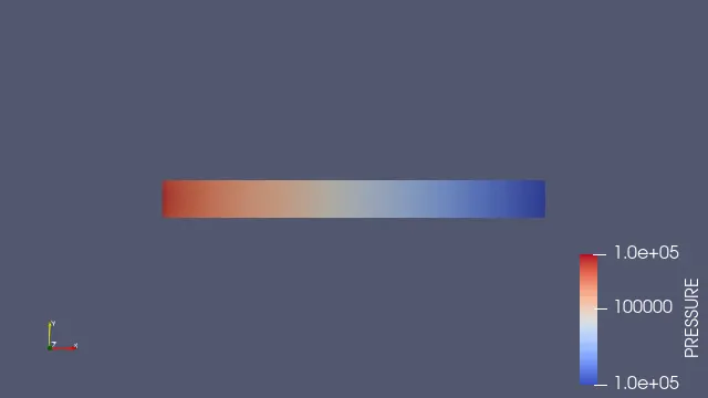
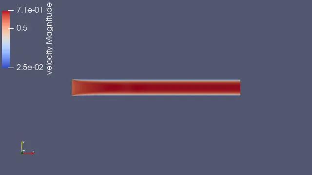
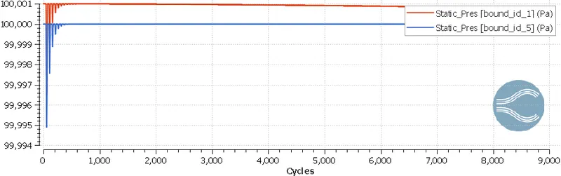
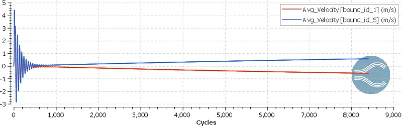
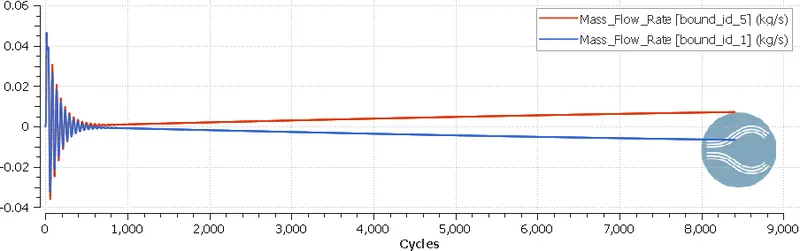
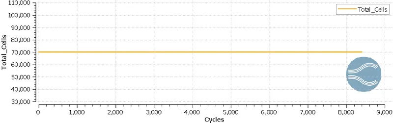
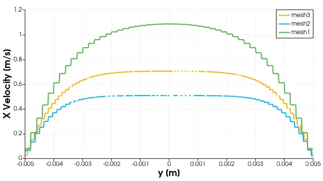
Velocity profile at outlet for all 3 cases:

Conclusion:

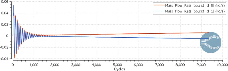
The development of flow seemed to have reached steady state from the velocity animations. Mass-flow rate plots also show similar inference with same inflow and outflow rates for all cases. Since this is a steady state simulation, the flow development shown is animation doesn't exactly represent the transient flow development in the duct.However, the development of mass fraction of n2 is clearly visible in a space filled with different mass fraction of n2. The animation of species mass-fraction shows that the effect of initial condition is being wiped out by the incoming fluid flow. However this process is not complete and steady state is yet to be reached in terms of species distribution. Since the steady state monitors created are not able to judge the developing species distribution in the domain, the case will need more iterations without convergence checking until the whole domain is filled with 73% nitrogen. Even though the resolution of velocity plots at outlet get better with increased cell count, the velocity plot in the coarse mesh is more realistic since it has achieved a better convergence state for species equation compared to the other two meshes. Providing a better initial condition, in this case species same as inflow, would help reach simulation reach a steady state much faster and the comparison between different meshes and their velocity profiles would make much more sense.