Week 1: Channel flow simulation using CONVERGE CFD

OBJECTIVE:

We are to run a simple channel flow simulation to test our setup and familiarise ourselves with CONVERGE basics. We will be simulating 3 cases:

• dx = 2e-4m, dy = 2e-4m, dz = 2e-4m
• dx = 1.5e-4m, dy = 1.5e-4m, dz = 1.5e-4m
• dx = 1.0e-4m, dy = 1.0e-4m, dz = 1.0e-4m

We will finally compare the results and document our observations.

INTRODUCTION:

This is a simple 2D channel flow simulation to test the converge installation and familiarise ourselves with it. We will compare the velocity and pressure contours across the three cases and comment on the changes if any.

SETUP:

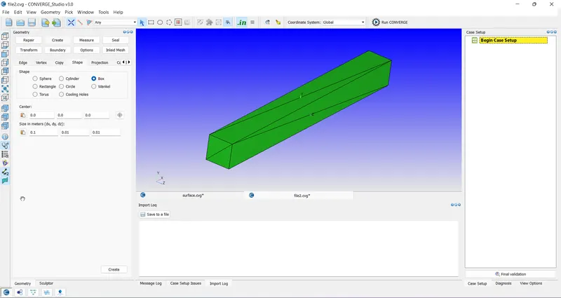
We will first create a Channel using the Create>Box tool, the dimensions are as follows:

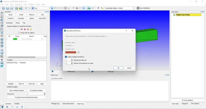
Then, we create the respective boundaries using the Boundary menu in Geometry box:

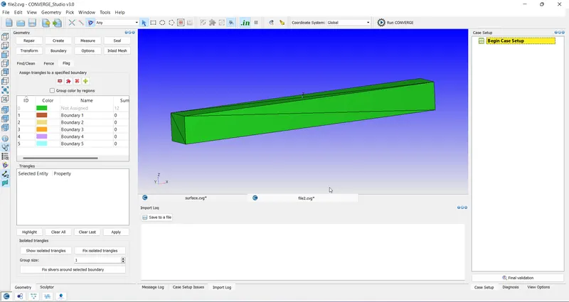
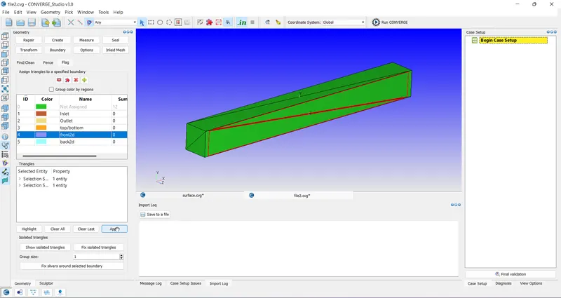
Once the Boundaries have been created, We assign them to the surfaces and rename them accordingly:

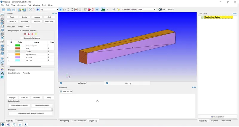
Moving on to the case setup, once we click on begin case setup, CONVERGE provides us with a menu based step-by-step process for setting up the case:

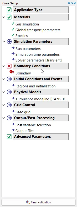
For our application we are choosing time-based:

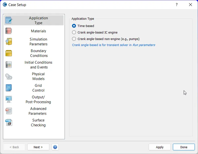
We will be using Air as the working fluid, hence AIr and Nitrogen will be chosen as species:

This is a steady-state simulation hence we will use a full hydrodynamic compressible steady-state solver enabled with a steady-state monitor and not using shared memory:

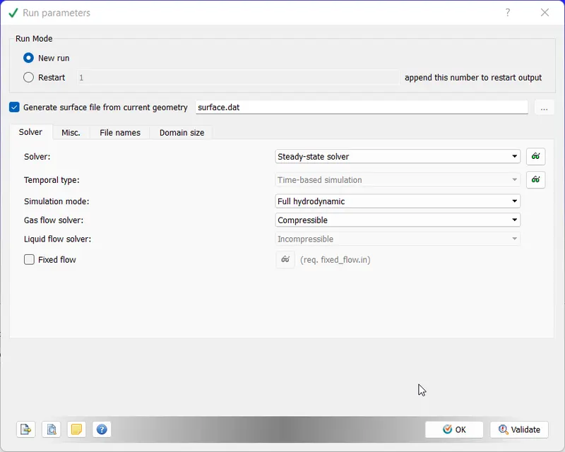
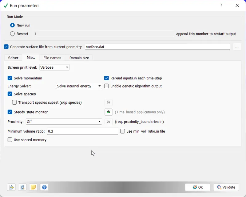
Next, we set up the time parameters including number of cycles and time step size:

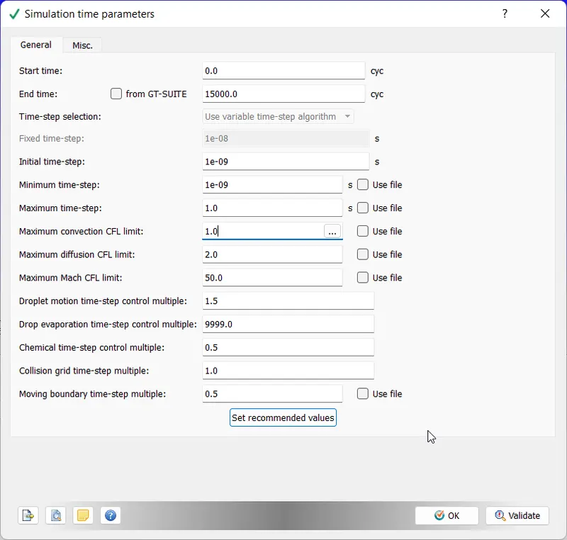
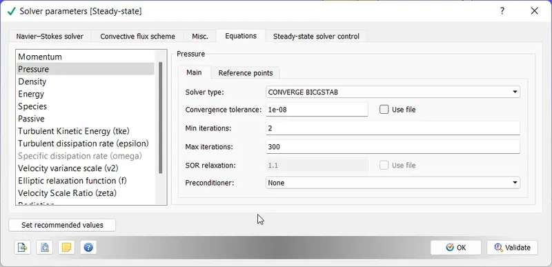
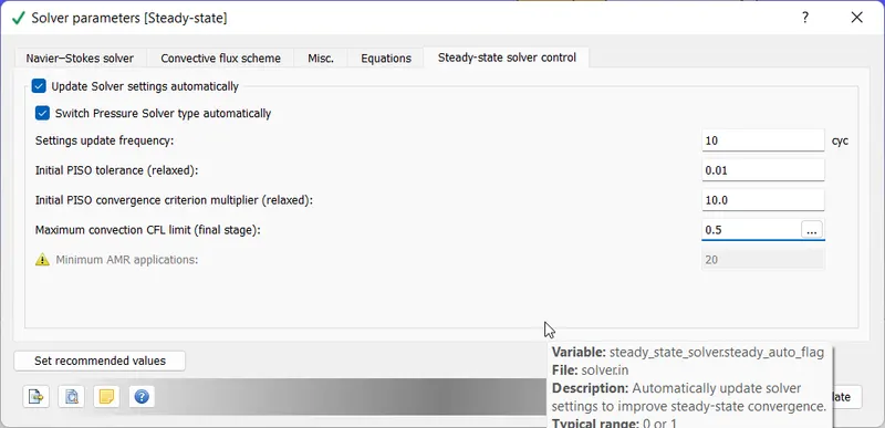
Next we set the Pressure Preconditioner to NONE and Maximum CFL number less than 1:

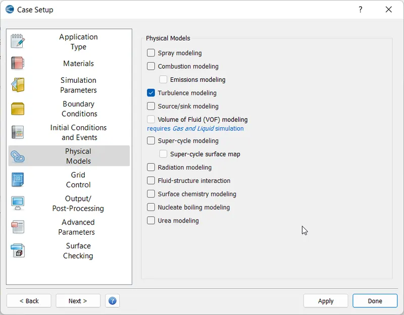
We will disable turbulence modelling for this particular case:

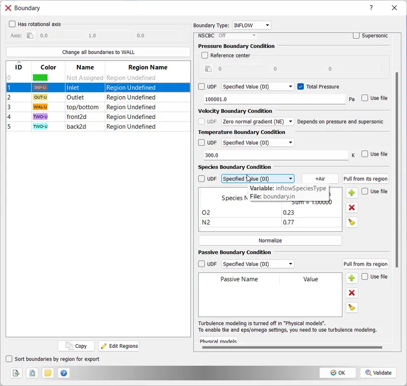
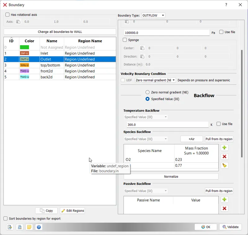
Then we will set the boundary conditions as follows:

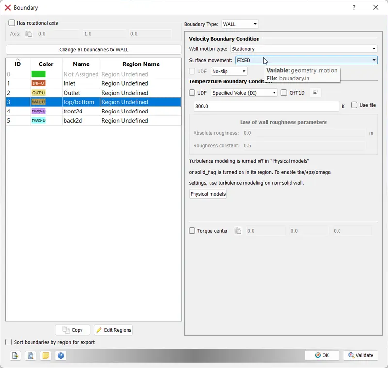
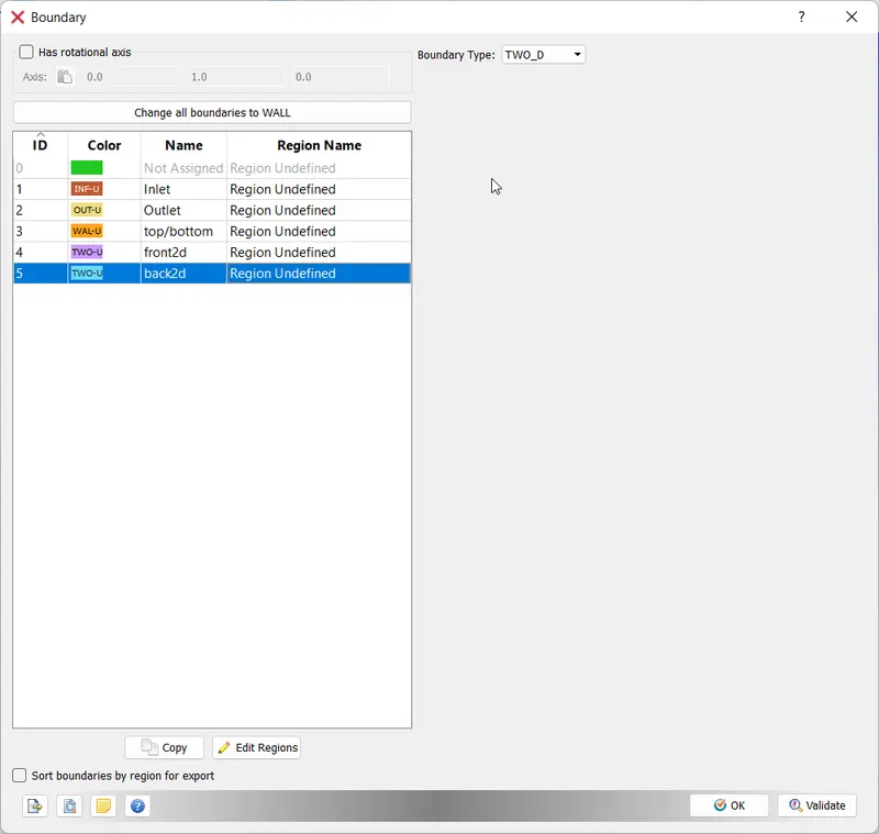
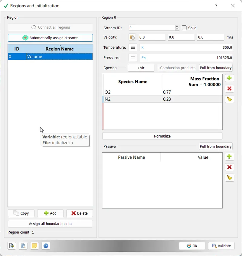
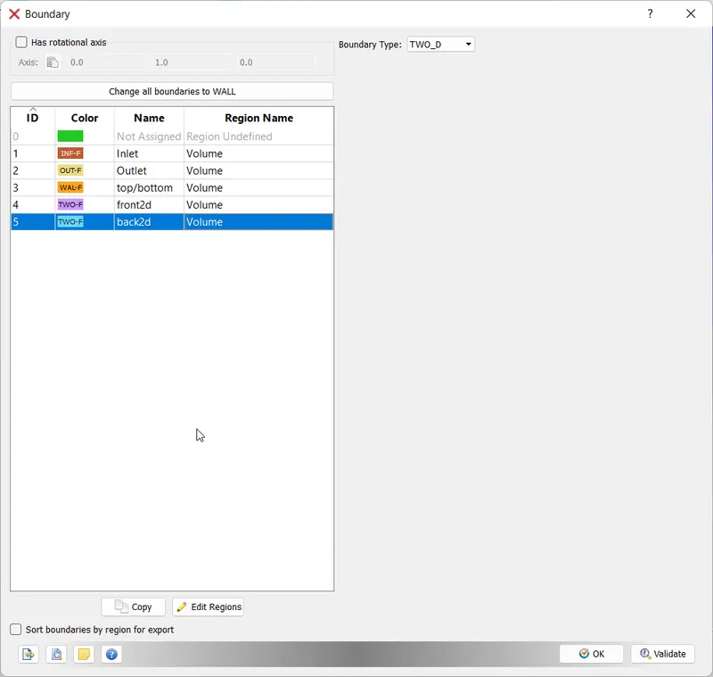
We will create a volumetric Region and set initial conditions, then assign the region to the boundaries:

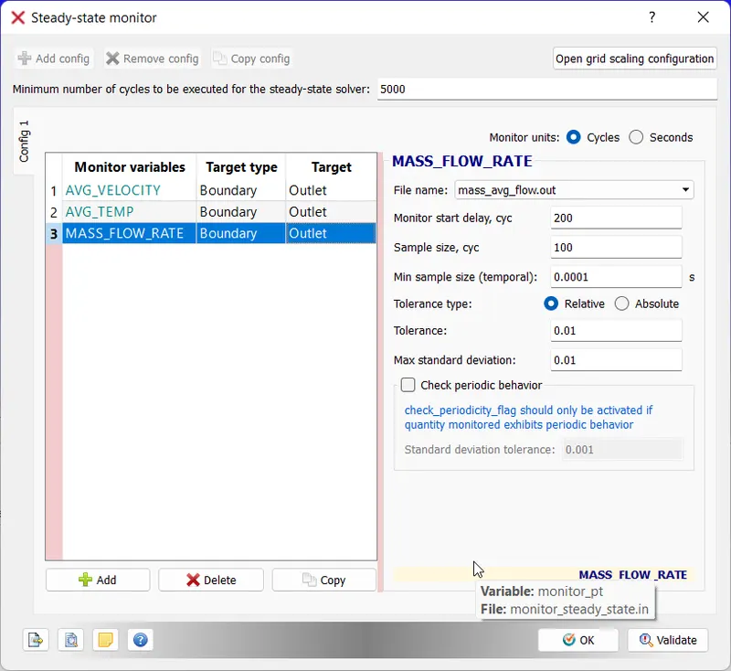
We will set-up a steady state monitor, for the following three variables and ensure that the simulation runs for at least 5000 cycles to get substantial information for result processing:

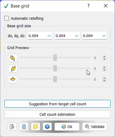
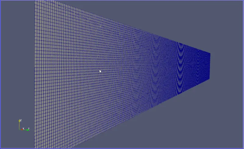
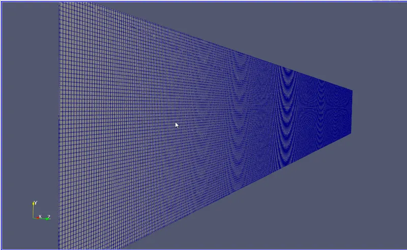
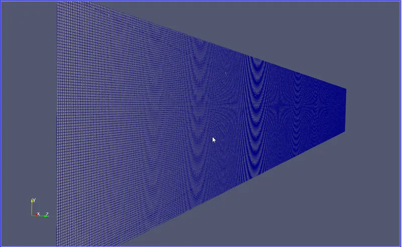
The grid will be set according to the objective, we will have three different cases based on the 3 provided grid sizes:

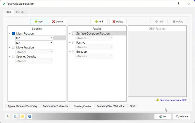
Finally, we will select the variables we are focusing our study on:

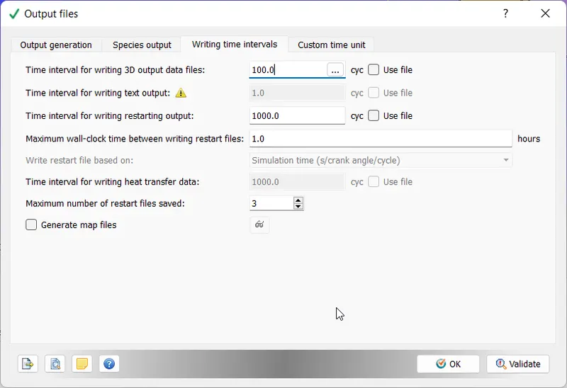
and set the limit on how many output files need to be written/cycle:

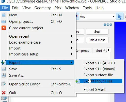
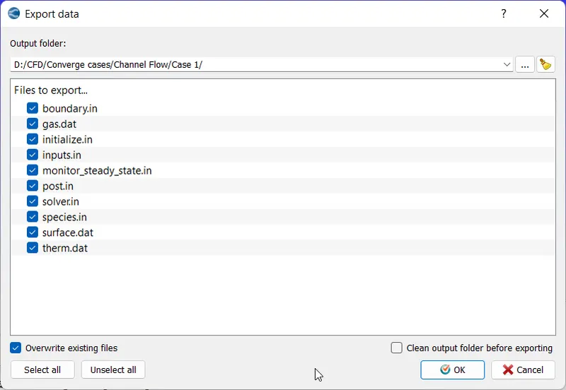
Once we have done the setup, we can now export the input files:

PROCESSING:

Once our case is set up we can execute it using the command line and mpiexec executable using the following command:

mpiexec.exe -n 4 converge.exe restricted

This will perform the numerical analysis on our input files and store the results in an output folder. Once the process is complete, we will have to post-convert the output to be able to post-process them.

To do this navigate to the output folder and run the post_convert executable:

mpiexec.exe -n 4 post_convert.exe

This will generate a group of *.vtm files which we can open in ParaView to post-process the results.

RESULTS:

CELL COUNT:

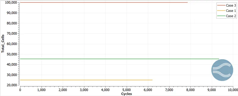
This plot shows the cell count of each case as well as the number of cycles it took to reach convergence.

CASE I:

Grid Size - 2e-4:

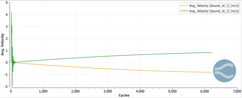
Velocity Plot:

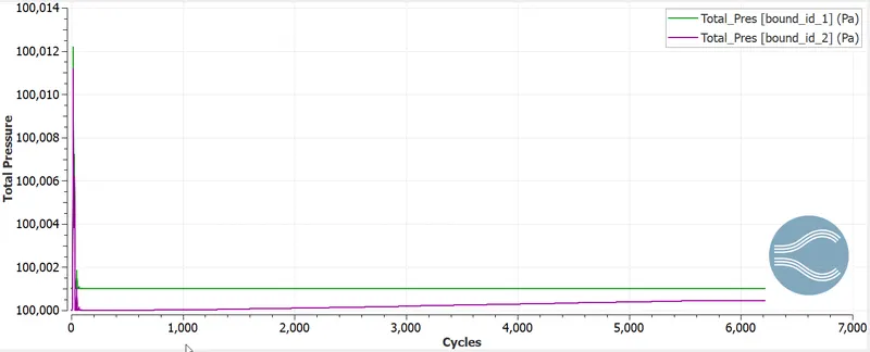
Pressure Plot:

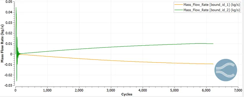
Mass Flow Rate:

CASE II:

Grid Size - 1.5e-4:

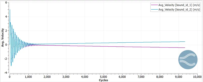
Velocity Plot:

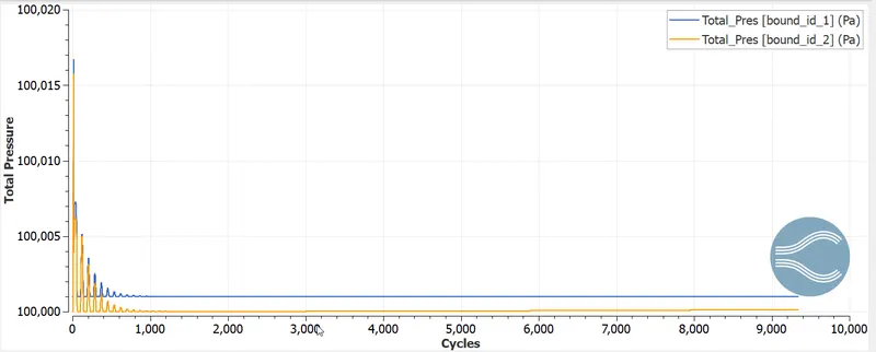
Pressure Plot:

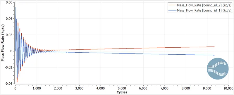
Mass Flow Rate:

CASE III:

Grid Size - 1e-4:

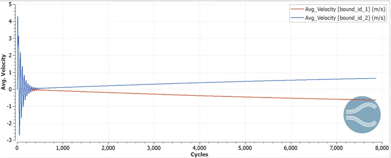
Velocity Plot:

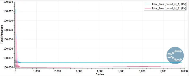
Pressure Plot:

Mass Flow Rate:

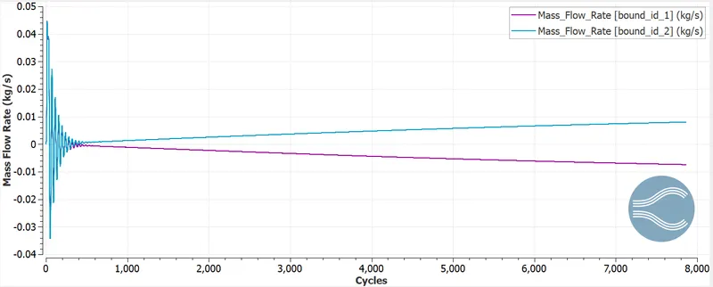
As we see from the plots, there is a negligible difference in the magnitudes of corresponding values which is to be expected since the case has been run for similar conditions.

The only obvious change can be observed in the animations where the flow gets more resolved near the walls as the mesh becomes finer.

CONCLUSION:

• There is some initial instability due to the initialization of the problem, the longer the solution's initial condition takes to stabilise the larger number of cycles are required to reach convergence.
• Lower grid size increases the simulation resolution as the region of low velocity near the walls decreases in size as we decrease the mesh size.