Using Simulink, plot a given function and run Simulink example “Suspension System Comparison”.

Objective:

1. To plot a Function y(x) = (x-1) * (x-3)^2 * (x-9)^2 using basic Simulink blocks.
2. To run Simulink example “Suspension System Comparison”.

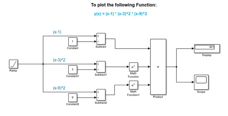
To plot a Function y(x) = (x-1) * (x-3)^2 * (x-9)^2 using basic Simulink blocks.

Simulink blocks used:

Ramp:

The Ramp block generates a signal that starts at a specified time and value and changes by a specified rate. The block's Slope, Start time, and Initial output parameters determine the characteristics of the output signal.

Constant:

The Constant block generates a real or complex constant value signal. Use this block to provide a constant signal input.

Subtract:

The Subtract block performs subtraction on its inputs. This block can subtract scalar, vector, or matrix inputs.

Math Function:

The Math Function block performs numerous common mathematical functions. For example, Exp, log,10^u, log10, |u|², square, reciprocal, mod, transpose, Hermitian etc.

Product block:

The Product block outputs the result of multiplying two inputs: two scalars, a scalar and a non-scalar, or two non-scalars that have the same dimensions.

Display Block:

The Display block shows the value of the input data.

Scope:

Scope block display signals generated during simulation.

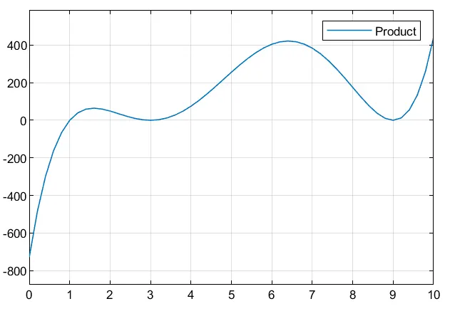
Scope Result:

To run Simulink example “Suspension System Comparison”.

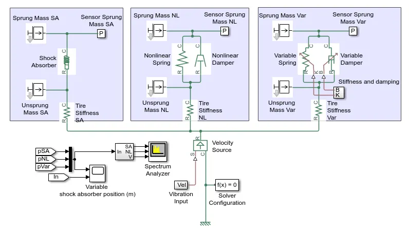
Results:

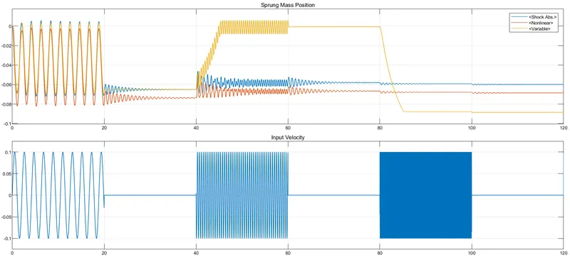
Introduction:

A vibratory system, in general, includes a means for storing potential energy (spring or elasticity), a means for storing kinetic energy (mass or inertia), and a means by which energy is gradually lost (damper).

The vibration of a system involves the transfer of its potential energy to kinetic energy and of kinetic energy to potential energy, alternately. If the system is damped, some energy is dissipated in each cycle of vibration and must be replaced by an external source if a state of steady vibration is to be maintained.

Objective of the Simulation:

The objective of the example is to compare the performance of three different types shock absorbers or ‘Spring and damper’ system which are excited by a velocity source.

Similarities and difference between the three systems under study:

The first system, uses the shock absorber block and includes linear stiffness and damping. The second system, uses a non-linear translational spring and a non-linear translational damper. The third, uses a variable translational spring and variable translational damper.

All the suspension systems are excited by the same velocity source. Tire stiffness, sprung mass and un-sprung mass are also same for all three systems.

Note: -

Sprung weight transfer is the weight transferred by only the weight of the vehicle resting on the springs, not the total weight of the vehicle.

Un-sprung weight transfer is calculated based on the weight of the vehicle’s components that are not supported by the springs. This includes tires, wheels, brakes. Spindles, half the control arm’s weight and other components.

Observations from the results:

In the simulation, all the three suspensions are excited by a velocity source. Since a damper/ dashpot is attached in all three cases. That means it is a case of forced damped vibration. We know that in force vibration, either we can apply a constant external force (step input forcing) or we can apply a harmonic force (Harmonic forcing).

For this exercise, harmonic force is applied that means external force or velocity source varies as “F sin (ω t)”. Here, maximum amplitude of force, F = 0.1 at sin (90). The velocity source is producing excitation in three stages over a total time interval of 120 seconds. All the excitations are produced for 20 seconds. After the 20 second excitation (harmonic force), additional 20 seconds are provided so that the system can damp out the vibration caused. First excitation is produced for 0-20 seconds. Second excitation is produced for 40-60 seconds. And, third excitation is produced for 80-100 seconds.

We can observe from the plot that, in all the three stages the time period and amplitude of harmonic force is constant but the frequency of harmonic force varies. For first stage, the frequency of harmonic force is least whereas for the 3^rd stage the frequency of harmonic force is highest.

Before we go into analysis, we should recall, at lower velocity, the Damping force is proportional to velocity, i.e., Fd = C * V. where C = damping coefficient. V = velocity. So higher the velocity or frequency of excitation, then higher will be the damping force. At higher velocity or frequency of excitation, the Damping force is proportional to square of velocity.

Case 1: Time period 0-40 seconds on time axis.

Here for 1^st 20 seconds, harmonic force is applied. And for 20-40 seconds the vibrations are allowed to damp out. The frequency of excitation is least in this case.

When the excitation is provided for 0-20 seconds to the suspensions, all suspensions along with the mass oscillate. The amplitude of oscillation is same in all the suspensions, during the excitation.

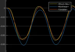
For time period 20-40 seconds, excitation stops and the vibrations are allowed to damp out. For variable suspension the vibration ends instantly, hence it has little or no amplitude of vibration. For shock absorber and non-linear suspension, the amplitude of vibration reduces gradually. Amplitude of vibration reaches zero, at around 35 seconds for shock absorber and at 37 seconds for non linear suspension. We can clearly see that the amplitude of vibrations is greater in cases of non-linear suspension followed by shock absorber.

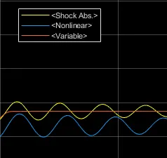
Hence, we can say that at given frequency and amplitude of vibration, the variable suspension will provide no cushioning effect since the vibration dies instantly. The non-variable suspension provides relatively more amplitude of vibration and it takes longer time for amplitude of vibration to subdue in comparison to shock absorber. Hence shock absorber is best choice in this case followed by non-linear suspension.

Case 2: Time period 40-80 seconds on time axis.

Frequency of excitation is higher in this case. Whereas the Amplitude of excitation remains the same.

During the Forced excitation period, of 20 seconds i.e., between 40-60 seconds on time axis. Due to higher frequency of excitation the suspensions are unable to stretch to their original length. As soon as the suspensions try to regain their original length the higher frequency excitation acts on them. Also, at higher frequency the damper offers higher resistance. As a result, the amplitude of vibration is lower in all the three suspensions system during excitation period when we compare it with case 1. The variable suspension deviates from its position due to variable property of its spring and damper, and attains constant amplitude after certain interval. The variable suspension has highest amplitude in this case followed by shock-absorber and Variable suspension. Obviously, at this frequency of excitation the cushioning effect will be less.

During the period 60-80 seconds on time axis, the vibrations caused are allowed to diminish. For variable suspension the vibration ends instantly, hence it has little or no amplitude of vibration. For shock absorber and non-linear suspension, the amplitude of vibration reduces gradually.

Clearly, during the period of force excitation (i.e., 40-60 seconds) the Variable suspension will provide more cushioning effect as it is absorbing more energy followed by shock-absorber and non-linear suspension. For next 20 seconds (i.e., 60-80 seconds), shock-absorber is producing more amplitude and the vibrations dies gradually. Hence looking at overall picture the shock absorber is better choice, compared to other two.

Case 3: Time period 80-120 seconds on time axis.

Frequency of excitation is highest in this case. Whereas the Amplitude of excitation remains the same.

During the Forced excitation period, of 20 seconds i.e., between 80-100 seconds on time axis. Due to higher frequency of excitation the suspensions are unable to stretch to their full length. As soon as the suspensions try to regain their full length the higher frequency excitation acts on them. As a result, the amplitude of vibration is lower in all the three suspensions system during excitation period when we compare it with case 1 and 2. The amplitude of vibration is least in case of Variable suspension. Whereas the performance of shock-absorber and non-linear suspension is very similar.

During the period 80-120 seconds on time axis, the vibrations caused are allowed to diminish. For variable suspension the vibration ends instantly, hence it has little or no amplitude of vibration. For shock absorber and non-linear suspension, the amplitude of vibration reduces gradually.

Hence, for this case, shock-absorber and non-linear suspension gives similar results and perform better than variable suspension system.

How the oscillating velocity source is created?

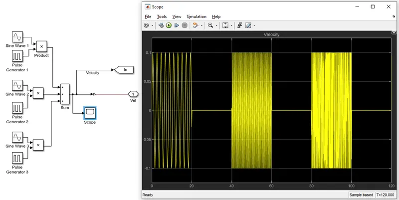
Velocity source is created by adding ‘sine wave’ block and ‘Pulse generator’ block. As shown below.

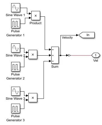
The ‘Sine wave 1’ block generates sine wave with an amplitude 0.1 with frequency 3 for 120 seconds time period.

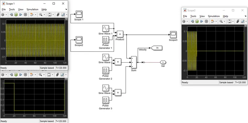
The ‘Pulse generator 1’ block generates square wave pulses with an amplitude of 1 and Phase delay of 0 seconds. Time period is 120 seconds. Pulse width is 16.666 % of Time period. Hence it will generate 1 square wave pulse of amplitude 1 with a width of 20 units for 0-20 seconds. Afterwards it will generate a straight line about its mean.

After multiplication of ‘Sine wave 1’ and ‘Pulse generator 1’ the sine wave within square wave will remain and rest of the sine wave is replaced by a straight line generated by ‘Pulse generator 1’.

The ‘Sine wave 2’ block generates sine wave with an amplitude 0.1 with frequency 15 for 120 seconds time period.

The ‘Pulse generator 2’ block generates square wave pulses with an amplitude of 1 and Phase delay of 40 seconds. Time period is 120 seconds. Pulse width is 16.666 % of Time period. Hence it will generate 1 square wave pulse of amplitude 1 with a width of 20 units for 40-60 seconds. Afterwards it will generate a straight line about its mean.

After multiplication of ‘Sine wave 2’ and ‘Pulse generator 2’ the sine wave within square wave will remain and rest of the sine wave is replaced by a straight line generated by ‘Pulse generator 2’.

The ‘Sine wave 3’ block generates sine wave with an amplitude 0.1 with frequency 75 for 120 seconds time period.

The ‘Pulse generator 2’ block generates square wave pulses with an amplitude of 1 and Phase delay of 80 seconds. Time period is 120 seconds. Pulse width is 16.666 % of Time period. Hence it will generate 1 square wave pulse of amplitude 1 with a width of 20 units for 80-100 seconds. Afterwards it will generate a straight line about its mean.

After multiplication of ‘Sine wave 2’ and ‘Pulse generator 2’ the sine wave within square wave will remain and rest of the sine wave is replaced by a straight line generated by ‘Pulse generator 2’.

The sine wave, square wave before and after product can be seen by adding scope block, as shown below:

At last, all the resultant Amplitude waves after the product, are added to generate three sine wave patterns with intermittent straight line about the mean. The sine wave depicts periods of forced excitation for the simulation and the straight line shows a period during which no excitation is given to the suspension and the vibrations generated are allowed to damp out. The addition of the waves can be seen by adding scope as shown: