Simulating Pendulum’s transient motion in MATLAB using ode45 numerical solver
Aim- Simulating Pendulum’s transient motion in MATLAB using ode45 numerical solver
Objectives-
- To find the solution of pendulum's motion ODE using ode45.
- To plot the obtained results.
- To animate the obtained plots using loops.
Introduction-
We have a bob of mass ‘m’ connected by a massless rod of length ‘l’ to a pivot point so the pendulum is able to swing along an arc. Gravity and a damping force is acting on the pendulum.
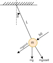
For motion along the arc only sin component of gravity is responsible.
Arc length is given by-
`s=lθ`
Velocity along the arc is given by-
`(ds)/dt=l(dθ)/dt`
Acceleration along the arc is given by-
`(d^2s)/dt^2=l(d^2θ)/dt`
From Newton’s Second law we can obtain-
`−mgsinθ−b(dθ)/dt=ml(d^2θ)/dt^2`
Thus a 2nd order non-linear ODE for pendulum obtained is-
`(d^2θ)/dt^2+b/(ml)(dθ)/dt+g/lsinθ=0`
Numerical ODE solver in MATLAB (ode45)-
The function ode45 is a numerical integrator solver in MATLAB that implements Runge-Kutta Method with a variable time step. It is designed to handle Initial value problems.
`dx/dt=f(t,x) ;x(t_0)=x_0`
Ode45 can only handle first order ODEs so for our case we reduced it down to two first order equations using required substitutions.
Let,
`theta=theta_1`
`(dθ)/dt=(dθ_1)/dt=θ_2`
`(d^2θ)/dt^2=(d^2θ_1)/dt^2=d/dt((dθ_1)/dt)=(dθ_2)/dt`
`(d^2θ_2)/dt^2+b/(ml)θ_2+g/lsinθ_1=0`
`d/dt[[θ_1],[θ_2]]=[[θ2],[−b/(ml)θ_2−g/lsinθ_1]]`
Coding in it-
[t,x]=ode45(@fname,tspan,xinit)">[t,x]=ode45(@fname,tspan,xinit)[t,x]=ode45(@fname,tspan,xinit)
- fname is the name of the function created in MATLAB script file for evaluation.
- tspan is the vector defining the starting and ending limits of integration.
- xinit is the vector of initial conditions.
- t is the value of independent variable at which solution array x is calculated.
- x is an array of solutions
CODE EXPLANATION-
- Initial Conditions for solving the ODE are initialised, limits for integration and physical properties of the pendulum are described.
clear all                               % Clears command history
close all                               % Closes  all windows
clc                                     % Clears command window
%=========================================================================
l=1;                                    %Length of string (m)
P=0.3;                                  %Mass of Bob (kg)
b=0.05;                                 %Damping Coefficient
g=9.81;                                 %Acceleration due to gravity (m/s2)
%==========================Initial Condition==============================
theta_0=[0;5];                          %INITIAL Angular displacement &
                                        %Angular Velocity
%===============================Time======================================
t_span=linspace(0,50,700);- For finding the solution MATLAB ode solver function ode45 is called and the ODE of the pendulum motion is called using the function ode_function. Moreover the coordinate values of the bob are calculated and stored in variables x, y, velocity of the bob is also calculated to simulate the vector using quiver function later on.
%=============================Solving ODE=================================
[t,results]= ode45(@(t,theta) ode_func(theta,b,g,l,P),t_span,theta_0);
[result1]=results(:,1);
[result2]=results(:,2);
o=[0,0];
x = l*sin(result1);
y =-l*cos(result1);
u = diff(x)./diff(t);
v = diff(y)./diff(t);
u = [u;0];
v = [v;0];- For making animated movie of the simulation VideoWriter function is used and a video handle vf is created with frame rate set to 25 fps.
%================================Animation================================

vf = VideoWriter('pendulum_simulation','mpeg-4');
vf.FrameRate=25;
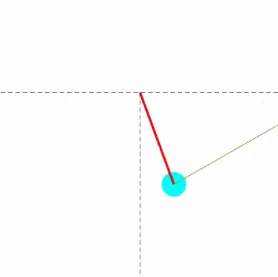
open(vf);- A figure window is being created named & window’s appearance is altered, measurement units were normalised where the lower-left corner of the container maps to (0, 0) and the upper-right corner maps to (1,1) thus the position of figure window was set to [0,0,1,1] to get a full-screen figure window. A for loop is used to plot the results obtained above with the help of ode45.
figure('units','normalized','outerposition',[0 0 1 1])

for i=1:length(t_span)

     subplot(1,2,1);
     a=plot(x(i),y(i),'co',[o(1),x(i)],[o(2),y(i)],'r-'...
             ,[-4,4],[0,0],'--k',[0,0],[0,-10],'k--');
     a(1).LineWidth=2;
     a(1).MarkerFaceColor='c';
     a(1).MarkerSize=30;
     a(2).LineWidth=3;
     hold on;
     quiver(x(i),y(i),u(i),v(i),'linewidth',1);
     hold off;
     axis('equal');
     axis([-1.5 1.5 -2 1]);
     pause(0.007);

     subplot(2,2,2)
     b=plot(result1(1:i),result2(1:i),...
         [0,0],[-10,10],'k--',[-5,5],[0,0],'k--',0,0,'o');
     b(1).LineWidth=2;
     grid on;
     axis([-2 2 -6 6])
     pause(0.007);

     subplot(2,2,4)
     c=plot(t(1:i),result1(1:i),t(1:i),result2(1:i),[0,50],[0,0],'k--');
     c(1).LineWidth=2;
     c(2).LineWidth=2;
     grid on;
     axis([0 50 -5 5])
     ylabel('Velocity & Displacement')
     xlabel('Time(sec)')
     title('Pendulum Oscillaitions')
     legend('Angular displacement','Angular velocity')
pause(0.007);- The frame generated after each iteration is being stored in a structure frames afterwards each frame is written in the video file using writeVideo, clf is used to clear figure window after each iteration ends.
frames=getframe(gcf);
     writeVideo(vf,frames);
     clf;


end
    close(vf);
Function ode_func script file for pendulum's behaviour-
function [dtheta_dt]=ode_func(theta,b,g,l,m)
    theta1=theta(1);
    theta2=theta(2);
    dtheta1_dt=theta2;
    dtheta2_dt=-(b/m*l)*theta2-(g/l)*sin(theta1);
    dtheta_dt=[dtheta1_dt;dtheta2_dt];
end
SCRIPT-
clear all                               % Clears command history
close all                               % Closes  all windows
clc                                     % Clears command window
%=========================================================================
l=1;                                    %Length of string (m)
P=0.3;                                  %Mass of Bob (kg)
b=0.05;                                 %Damping Coefficient
g=9.81;                                 %Acceleration due to gravity (m/s2)
%==========================Initial Condition==============================
theta_0=[0;5];                          %INITIAL Angular displacement &
                                        %Angular Velocity
%===============================Time======================================
t_span=linspace(0,50,700);
%=============================Solving ODE=================================
[t,results]= ode45(@(t,theta) ode_func(theta,b,g,l,P),t_span,theta_0);
[result1]=results(:,1);
[result2]=results(:,2);
o=[0,0];
x = l*sin(result1);
y =-l*cos(result1);
u = diff(x)./diff(t);
v = diff(y)./diff(t);
u = [u;0];
v = [v;0];
%================================Animation================================

vf = VideoWriter('pendulum_simulation','mpeg-4');
vf.FrameRate=25;
open(vf);

figure('units','normalized','outerposition',[0 0 1 1])

for i=1:length(t_span)

     subplot(1,2,1);
     a=plot(x(i),y(i),'co',[o(1),x(i)],[o(2),y(i)],'r-'...
             ,[-4,4],[0,0],'--k',[0,0],[0,-10],'k--');
     a(1).LineWidth=2;
     a(1).MarkerFaceColor='c';
     a(1).MarkerSize=30;
     a(2).LineWidth=3;
     hold on;
     quiver(x(i),y(i),u(i),v(i),'linewidth',1);
     hold off;
     axis('equal');
     axis([-1.5 1.5 -2 1]);
     pause(0.007);

     subplot(2,2,2)
     b=plot(result1(1:i),result2(1:i),...
         [0,0],[-10,10],'k--',[-5,5],[0,0],'k--',0,0,'o');
     b(1).LineWidth=2;
     grid on;
     axis([-2 2 -6 6])
     pause(0.007);

     subplot(2,2,4)
     c=plot(t(1:i),result1(1:i),t(1:i),result2(1:i),[0,50],[0,0],'k--');
     c(1).LineWidth=2;
     c(2).LineWidth=2;
     grid on;
     axis([0 50 -5 5])
     ylabel('Velocity & Displacement')
     xlabel('Time(sec)')
     title('Pendulum Oscillaitions')
     legend('Angular displacement','Angular velocity')
     pause(0.007);

     frames=getframe(gcf);
     writeVideo(vf,frames);
     clf;


end
    close(vf);
Results and Conclusion-
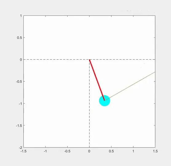
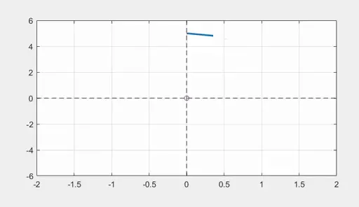
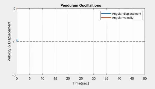
Thus, the pendulum's motion is simulated and animated successfully in MATLAB.
References-
- http://www.eng.auburn.edu/~tplacek/courses/3600/ode45berkley.pdf
- https://www.12000.org/my_notes/matlab_ODE/
- http://www.ece.northwestern.edu/local-apps/matlabhelp/techdoc/ref/ode45.html
- http://www.dtc.ox.ac.uk/online-learning/matlab/SolvingODEsInMatlab/UsingMatlabForSolvingODEsInitialValueProblems.xhtml
- https://ocw.mit.edu/resources/res-18-009-learn-differential-equations-up-close-with-gilbert-strang-and-cleve-moler-fall-2015/solving-odes-in-matlab/ode45/