Aim-Optimization using Genetic Algorithm in MATLAB®

Objectives-

• 1. Global Maxima of Stalagmite Function will be measured
• 2. Data sets will be devised for giving inputs to Genetic Algorithm for optimization.
• 3. Data from the set will be synthesised for plotting the stalagmite function.
• 4. Optimization will be done for three cases namely-
• a) With un-constrained inputs
• b) With constrained Lower & Upper bounds
• c) With constrained input and increased population size

Introduction-

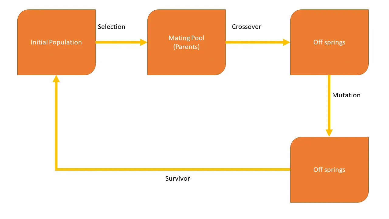
Genetic algorithms are evolutionary algorithms, which are based on natural selection & genetics. GAs use Darwin’s Theory of Survival of the fittest to evolve to an optimal solution. It selects individuals at random from the population to mate and produce off springs. In every generation, the artificially generated off springs mutate and over a few generations it converges to an optimal solution.

• Genetic Algorithms have been developed by John Holland and his acquaintances in University of Michigan, Ann Harbour.
• The main idea behind GA is robustness, i.e. whichever solution is fit for survival in many different environments is allowed to transfer data to another generation & vice-versa.
• Genetic Algorithm can be applied to solve a variety of optimization problems that are discontinuous, highly non-linear & non-differentiable.

Working Principle-

• Step 1-Initialize, create a population of N elements each randomly generated.
• Step 2- Selection, evaluate fitness of each element of population and build a mating pool.
• Step 3- Reproduction
  • Pick two parents from the population according to their fitness
  • Crossover
  • Mutate
  • Add new child to the population
• Step 4- Replace old population with new population and return to Step 2.

Genetic Algorithm Solver MATLAB-

“ga” is a function which determines the minimum of a function using genetic algorithm.

Syntax-

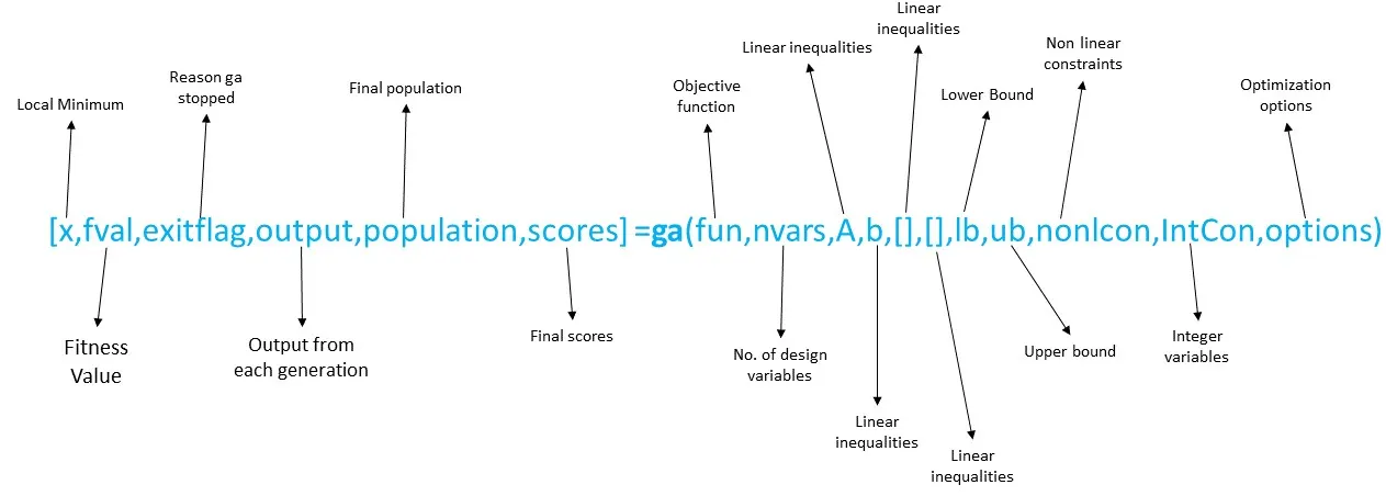
• fun — Objective function
• nvars — Number of variables
• A, b — Linear inequality constraints of type A*x <= b
• Aeq, Beq — Linear equality constraints of type Aeq*x = beq
• Bounds- lb ub
• nonlcon —(Nonlinear constraints) a function that accepts a vector or array x and returns two arrays, c(x) and ceq(x).
  • c(x) is the array of nonlinear inequality constraints at x
  • ceq(x) is the array of nonlinear equality constraints at x
• options — Optimization options output of optimoptions

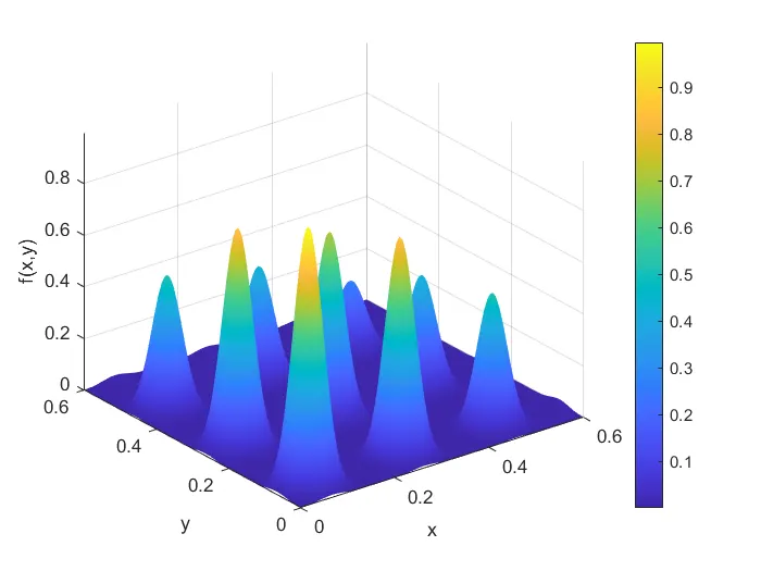
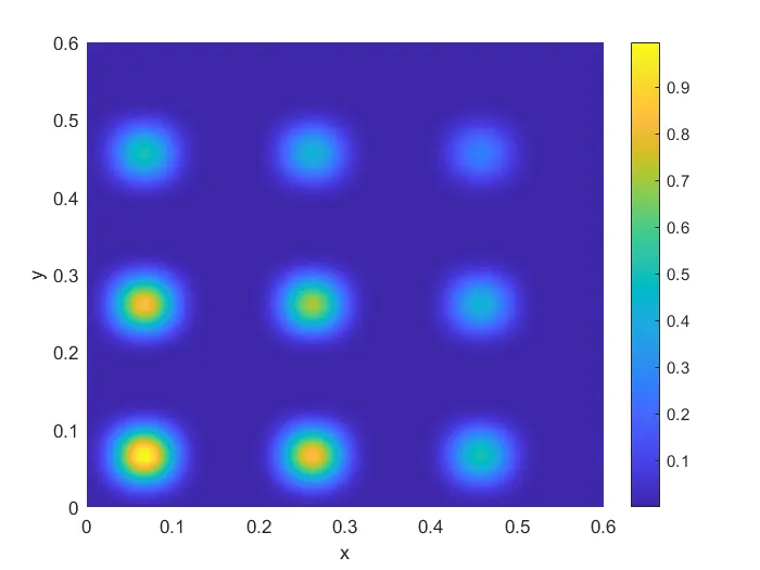
Stalagmite Function-

A stalagmite is a type of rock formation that rises from the floor of a cave due to the accumulation of material deposited on the floor from ceiling drippings.

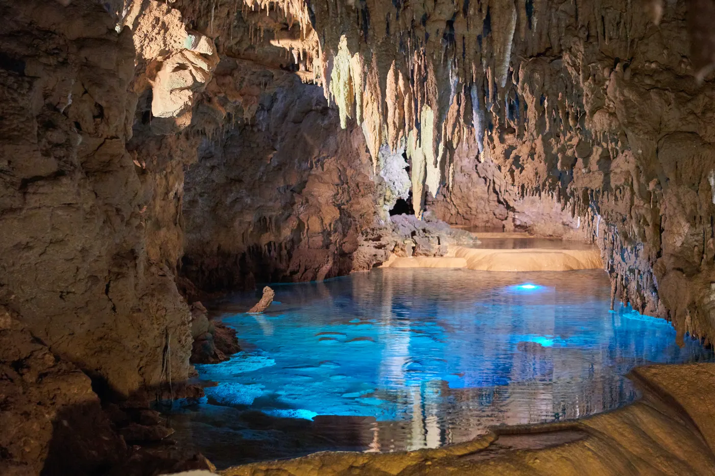
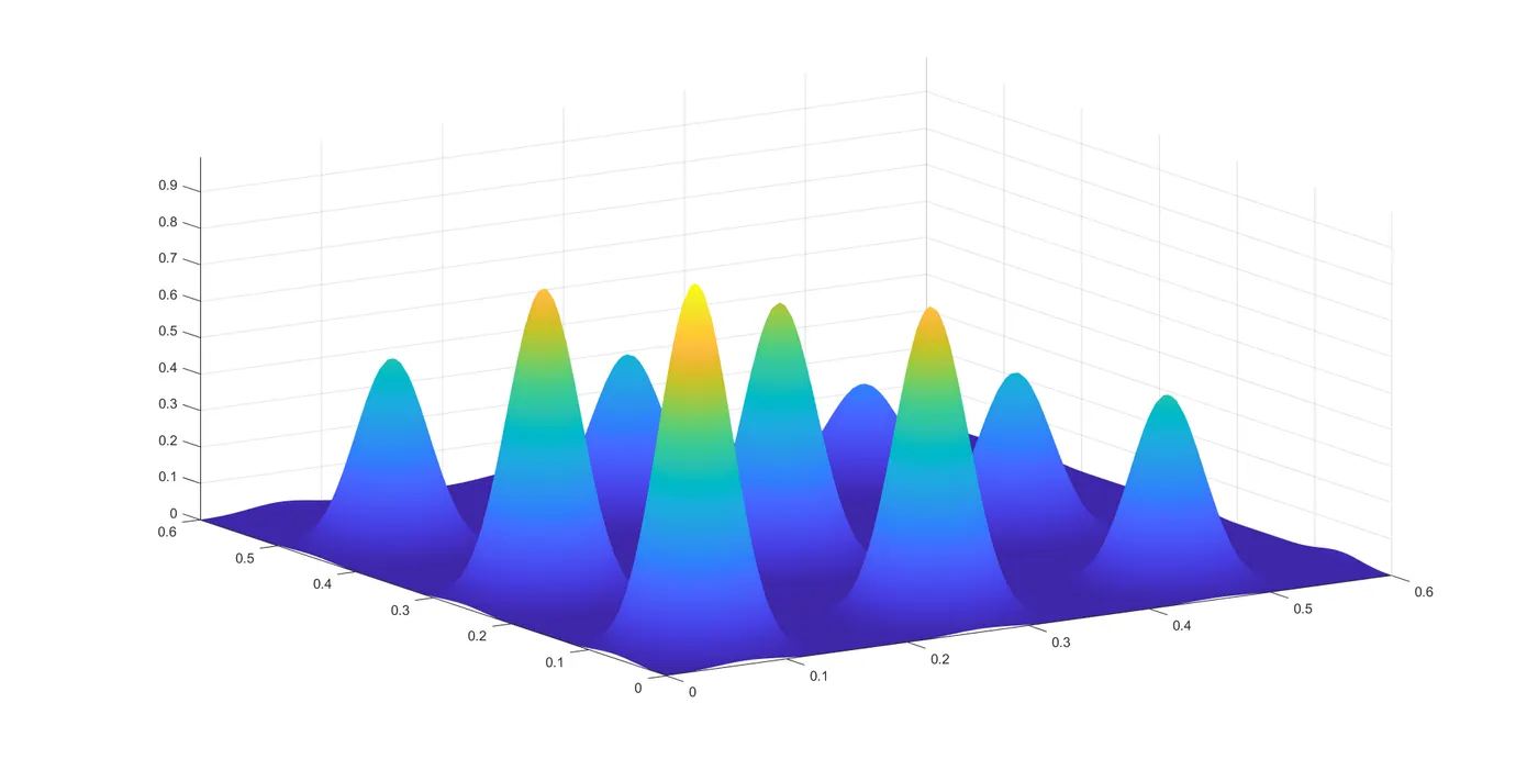
Mathematically we can model stalagmites as

`f(x,y)=f_(1x).f_(1y).f_(2x).f_(2y)`

Where,

• `f_(1x)=sin⁡((5.1πx+0.5))^6`
• `f_(1y)=sin⁡((5.1πy+0.5))^6`
• `f_(2x)=e^{-4 ln⁡2 (x-0.0667)^2/0.64}`
• `f_(2y)=e^{-4 ln⁡2 (y-0.0667)^2/0.64}`

`f(x,y)=sin⁡((5.1πx+0.5))^6 .sin⁡((5.1πy+0.5))^6 .e^{-4 ln⁡2 (x-0.0667)^2/0.64} .e^{-4 ln⁡2 (y-0.0667)^2/0.64}`

Objective function(stalagmite.m)-

%% ==================Stalagmite objective function=========================
function [Y]= stalagmite(X)
x=X(1);                                                         %Variable 1      
y=X(2);                                                         %Variable 2

f1x= sin(5.1.*pi.*x+0.5).^6;
f1y= sin(5.1.*pi.*y+0.5).^6;

f2x= exp((-4.*log(2)).*((x-0.0667).^2/0.64));
f2y= exp((-4.*log(2)).*((y-0.0667).^2/0.64));

f=(f1x*f1y*f2x*f2y);
Y=-f;                               %Minus sign is added to evaluate MAXIMA

end
%==========================================================================

Code Explanation-

1. Optimization of Stalagmite function using GA in an unbound manner-

• Initializing the search space for the genetic algorithm to work upon, meshgrid is used for creation of

• %% =============== Preparing the Search Space==============================
  x=linspace(0,0.6,150);                             % X-values
  y=linspace(0,0.6,150);                             % Y-values
  %================2D array creation using meshgrid Function=================
  [X,Y]=meshgrid(x,y);
  func= zeros;
  for i=1:length(X)
      for j=1:length(Y)
          input(1)=X(i,j);
          input(2)=Y(i,j);
          func(i,j)=stalagmite(input);
      end
  end

• Now, GA is employed for finding optimal solution with no. of iterations to be governed by 'num_case'. Furthermore stalagmite function is plotted, tic-toc commands are used for stuying the execution time of GA and subplot for maximum function value vs no. of iterations.

• num_case=30;
  %% ----------------------Unbound optimization------------------------------
  figure(1)
  surfc(X,Y,-func)
  shading interp
  xlabel('x');
  ylabel('y');
  zlabel('f(x,y)');
  
  tic
  objfunc=@stalagmite;                                    %objective function
  for k=1:num_case
      [maxima,f_opt(k)]=ga(objfunc,2);
      x_opt(k)=maxima(1);
      y_opt(k)=maxima(2);
  end
  a=toc;
  
  figure(2)
  subplot(2,1,1)
  
  surfc(X,Y,-func)
  xlabel('x');
  ylabel('y');
  zlabel('f(x,y)');
  title('Unbound Optimization');
  shading interp
  hold on 
  plot3(x_opt,y_opt,-f_opt,'marker','o','markersize',6,'markerfacecolor','r');
  
  subplot(2,1,2)
  plot(abs(f_opt))
  xlabel('No.of Iterations');
  ylabel('Max. Function Value');
  

• For each iteration we are getting optimal maxima(f_opt) of the stalagmite fucntion along with optimal design parameters(x_opt,y_opt).

2. Optimization of Stalagmite function using GA in a bound manner-

• Now this part of the code deals with the bound optimization with lower & upper bounds, thus the GA syntax is altered appropriately as per the defination of the stalagmite(objective function), lower bound of 0 and upper bound of 1 is initialized for improving the accuracy of GA, rest of the code remains same like the unbound case.

• %% =============Bound Optimization wtih upper and lower bounds=============
  tic
  for i=1:num_case
      [maximab,f_optb(i)]=ga(objfunc,2,[],[],[],[],[0;0],[1;1]);
      x_optb(i)=maximab(1);
      y_optb(i)=maximab(2);
  end
  
  b=toc;
  
  figure(3)
  subplot(2,1,1)
  
  surfc(X,Y,-func)
  shading interp
  xlabel('x');
  ylabel('y');
  zlabel('f(x,y)');
  title('Bound Optimization');
  hold on 
  plot3(x_optb,y_optb,-f_optb,'marker','o','markersize',6,'markerfacecolor','r');
  
  subplot(2,1,2)
  plot(abs(f_optb))
  xlabel('No.of Iterations');
  ylabel('Max. Function Value');
  

3. Optimization of Stalagmite function using GA in a bound manner with increased population size-

• To further increase the accuracy of GA we increase the population size of search space by using the optimoptions function.

• %% ================Increasing Population Size==============================
  options=optimoptions('ga');
  options=optimoptions(options,'PopulationSize',500);
  
  tic
  for i=1:num_case
      [maximaip,f_optip(i)]=ga(objfunc,2,[],[],[],[],[0,0],[1,1],[],[],options);
      x_optip(i)=maximaip(1);
      y_optip(i)=maximaip(2);
  end
  
  c=toc;
  
  
  
  figure(4)
  subplot(2,1,1)
  
  surfc(X,Y,-func)
  shading interp
  xlabel('x');
  ylabel('y');
  zlabel('f(x,y)');
  title('Bound Optimization with Increased population');
  hold on 
  plot3(x_optip,y_optip,-f_optip,'marker','o','markersize',6,'markerfacecolor','r');
  
  subplot(2,1,2)
  plot(abs(f_optip))
  xlabel('No.of Iterations');
  ylabel('Max. Function Value');
  ​ 

Main Script(genetic_algorithm_main.m)-

%------------------Genetic Algorithm Main Script---------------------------
clear all                                          % Clears command history
close all                                          % Closes  all windows
clc                                                % Clears command window
%% =============== Preparing the Search Space==============================
x=linspace(0,0.6,150);                             % X-values
y=linspace(0,0.6,150);                             % Y-values
%================2D array creation using meshgrid Function=================
[X,Y]=meshgrid(x,y);
func= zeros;
for i=1:length(X)
    for j=1:length(Y)
        input(1)=X(i,j);
        input(2)=Y(i,j);
        func(i,j)=stalagmite(input);
    end
end
num_case=30;
%% ----------------------Unbound optimization------------------------------
figure(1)
surfc(X,Y,-func)
shading interp
colorbar
%view(2)
xlabel('x');
ylabel('y');
zlabel('f(x,y)');

tic
objfunc=@stalagmite;                                    %objective function
for i=1:num_case
    [maxima,f_opt(i)]=ga(objfunc,2);
    x_opt(i)=maxima(1);
    y_opt(i)=maxima(2);
end
a=toc;

figure(2)
subplot(2,1,1)

surfc(X,Y,-func)
xlabel('x');
ylabel('y');
zlabel('f(x,y)');
title('Unbound Optimization');
shading interp
hold on 
plot3(x_opt,y_opt,-f_opt,'marker','o','markersize',6,'markerfacecolor','r');

subplot(2,1,2)
plot(abs(f_opt))
xlabel('No.of Iterations');
ylabel('Max. Function Value');


%% =============Bound Optimization wtih upper and lower bounds=============
tic
for i=1:num_case
    [maximab,f_optb(i)]=ga(objfunc,2,[],[],[],[],[0;0],[1;1]);
    x_optb(i)=maximab(1);
    y_optb(i)=maximab(2);
end

b=toc;

figure(3)
subplot(2,1,1)

surfc(X,Y,-func)
shading interp
xlabel('x');
ylabel('y');
zlabel('f(x,y)');
title('Bound Optimization');
hold on 
plot3(x_optb,y_optb,-f_optb,'marker','o','markersize',6,'markerfacecolor','r');

subplot(2,1,2)
plot(abs(f_optb))
xlabel('No.of Iterations');
ylabel('Max. Function Value');

%% ================Increasing Population Size==============================
options=optimoptions('ga');
options=optimoptions(options,'PopulationSize',500);

tic
for i=1:num_case
    [maximaip,f_optip(i)]=ga(objfunc,2,[],[],[],[],[0,0],[1,1],[],[],options);
    x_optip(i)=maximaip(1);
    y_optip(i)=maximaip(2);
end

c=toc;



figure(4)
subplot(2,1,1)

surfc(X,Y,-func)
shading interp
xlabel('x');
ylabel('y');
zlabel('f(x,y)');
title('Bound Optimization with Increased population');
hold on 
plot3(x_optip,y_optip,-f_optip,'marker','o','markersize',6,'markerfacecolor','r');

subplot(2,1,2)
plot(abs(f_optip))
xlabel('No.of Iterations');
ylabel('Max. Function Value');
%% ========================Displays the output=============================
%==========================================================================
disp(['Time Taken by Genetic Algorithm to optimize in unbound manner =' num2str(a),'sec'])
disp(['Time Taken by Genetic Algorithm to optimize in bound manner =' num2str(b),'sec'])
disp(['Time Taken by Genetic Algorithm to optimize in bound manner with Increased population =' num2str(c),'sec'])
%==========================================================================
disp(['MAXIMA of Stalagmite function when optimized in unbound manner =' num2str(max(-f_opt))])
disp(['MAXIMA of Stalagmite function when optimized in bound manner =' num2str(max(-f_optb))])
disp(['MAXIMA of Stalagmite function when optimized in bound manner with increased population =' num2str(max(-f_optip))])
disp(['MAXIMA of Stalagmite function lies at  x = ' num2str(maximaip(1)) ' y = ' num2str(maximaip(2))])


  

Results-

Unbound Optimization-

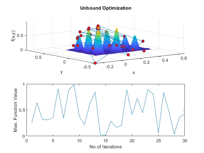
• From the graph and the table we can clearly see that in unbound manner GA predicts many local maxima as during the 30 iterations value gets changed at every iteration, thus low accuracy is obtained.

Bound Optimization-

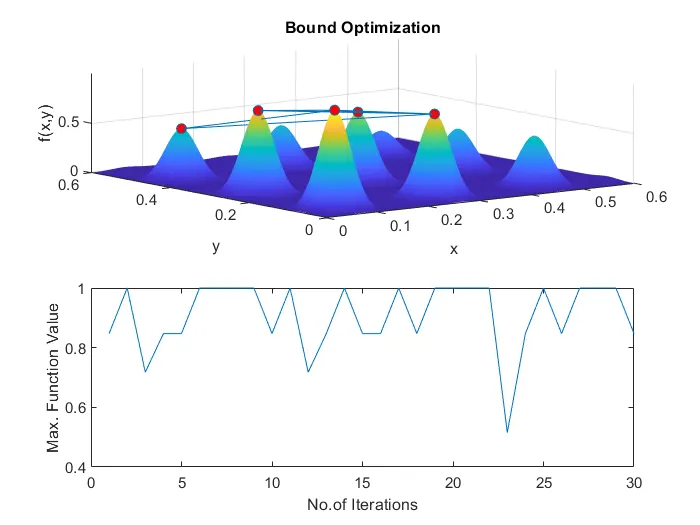
• In this case of bound optimization the accuracy is improved, it is clearly evident from the figures above.

Bound Optimization with increased population size-

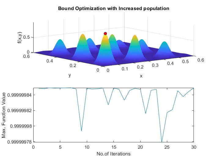
In this case the GA predicts only one maxima which is the global maxima for the stalagmite function, hence by bounding and increasing the population size we can increase the accuracy of the genetic algorithm.

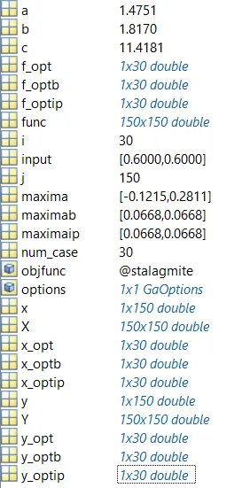
Workspace generated during the optimization process.

Conclusion-

• We used the genetic algorithm to optimize the stalagmite function & found that its Optimum maximum value is 1 which lies at

x=0.066832

y=0.033833

References-

1. Genetic Algorithms in Search, Optimization and Machine Learning by David E. Goldberg
2. Multi Objective Optimization using Evolutionary Algorithms by Kalyanmoy Deb
3. Genetic Algorithm and its Applications to Mechanical Engineering: A Review
4. Practical Genetic Algorithms in Python and Matlab By Yarpiz.com
5. Computer Aided Applied Single Objective Optimization By NPTEL IIT Guwahati
6. Genetic Algorithm Numerical Example by Zead Ibraheem
7. Genetic Algorithm By Prof.C.Balaji | IIT Madras
8. Genetic Algorithm Optimization By Alexander Robles