Aim-To simulate a planer robotic arm using Denavit-Hartenberg transformation in MatLab

Objectives-

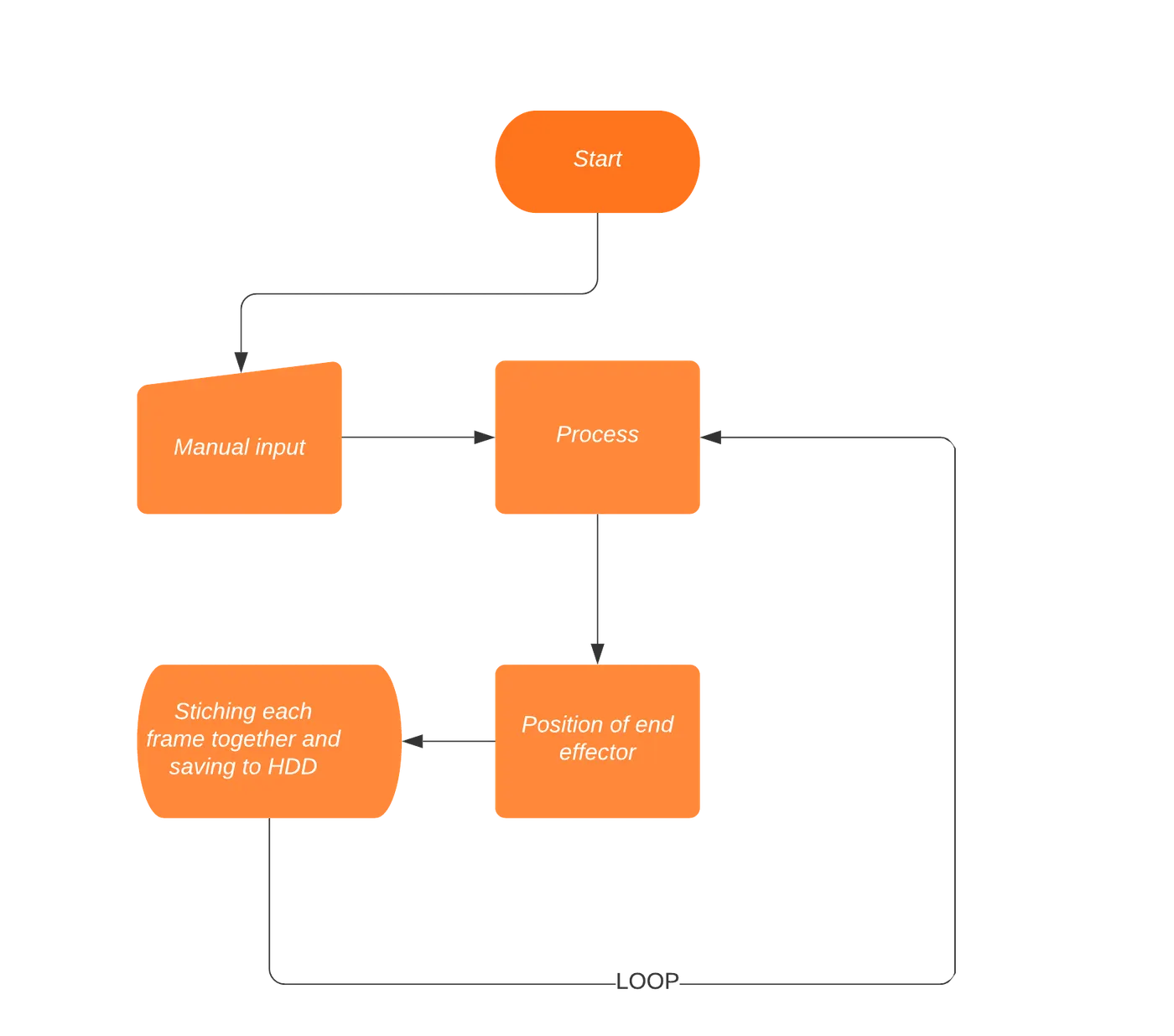
• To find the position of end effector using D-H method
• To change the values of joint variables and finding new position of end effector using LOOPS
• To plot the results of changed joint variables and end effector position
• To animate the obtained plots

Introduction

Robots have emerged as great alternatives for human workers for performing various engineering jobs but let’s go to the origin of this term. Robot, this word’s origin can be traced from the Czech word “robota” which means forced or compulsory labour.

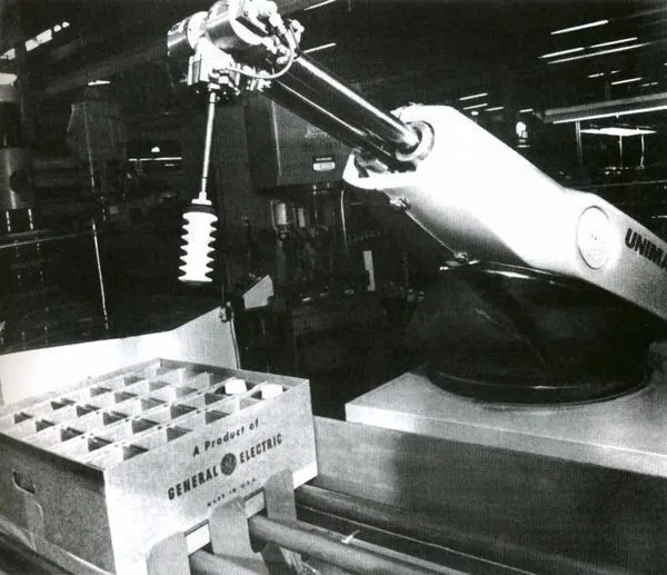
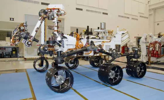
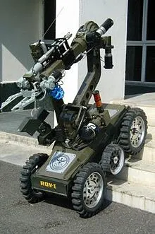
World’s first commercial, programmable robot was “Unimate” developed by George.C.Devol in 1958 later it was sold to GENERAL MOTORS Automobile Factory in New Jersey in 1961 & was tasked to perform automated die casting for car parts ,it had 6 DoF. Since then robots have evolved much and eased our work in different fields namely Welding,painting,inspection,agriculture,for nursing purpose,military,security,underwater, space explorations(MARS pathfinder Lander by NASA) and much more.

As per International Standard Organisation (ISO) 8373 a robot is formally defined as an “actuated mechanism programmable in two or more axes with a degree of ability to perform intended tasks based on current state and sensing, without human intervention”.

Denavit-Hartenberg Transformation method-

A robotic manipulator consists of links which are attached by either revolute or prismatic joints, in D-H method we tend to calculate the rotation matrix & displacement vector of the end-effector wrt the base frame in a recursive manner.

The method goes as follows-

• Step 1:- Assign the frames according to the D-H rules.
• Step 2:-Fill out the D-H parameter table.
• Step 3:-Plug the obtained parameters in the homogenous transformation matrix.

`[[cos⁡(θn),-sin⁡(θn)cos⁡(αn),sin⁡(θn) sin⁡(αn),rn cos⁡(θn)],[sin⁡(θn),cos⁡(θn)cos⁡(αn),-cos⁡(θn)sin⁡(αn),rn sin⁡(θn)],[0,sin⁡(αn),cos⁡(αn),dn],[0,0,0,1]]`

Rules for assigning D-H frames-

• Rule 1:- The Z-axis must be the axis of rotation of a revolute joint or dir. of motion for a prismatic joint.
• Rule 2:- The X-axis must be perpendicular both to its own Z-axis & the Z- axis of the frame before it.
• Rule 3:- All frames must follow right hand thumb rule.
• Rule 4:-Each X-axis must intersect the Z-axis of the frame before it.

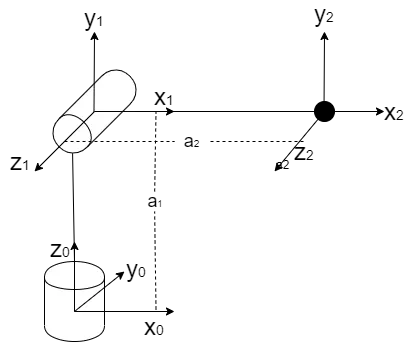
After keeping the rules in mind the kinematic diagram for the 2r manipulator is drawn as shown below

DH Parameter table-

n	Θ	α	r	d
1	Θ1	90	0	a1
2	Θ2	0	a2	0

• Θ is defined as the angle that is required to align x_n-1 to x_n wrt rotation about z_n-1.(But since x_n-1 and x_{n are} already aligned we simply put the value of joint variables (Θ_{1 &} Θ₂)).
• α is defined as the angle that is required to align z_n-1 to z_n wrt rotation about x_n. (Between frame 0 and 1 if z₀ is rotated about x₁ in 90⁰ anti-clockwise direction it will be aligned with z₁ while between frame 1 and 2 both z axes are aligned)

• r is defined as the distance between z_n-1 & z_n measured along x direction.

• d is defined as the distance between x_n-1 & x_n measured along z direction.

As the manipulator we are simulating is planer, the D-H parameter table is modified for 2D-

n	Θ	α	r	d
1	Θ1	0	l1	0
2	Θ2	0	l2	0

The homogeneous transformation matrix has the rotation matrix as well as displacement vectors for the frames, since our concern is about the 2D planer robotic arm so we will focus mainly on displacement vectors for the positions and will be neglecting the orientations from the rotation matrix, as in 2D orientation doesn’t make any sense.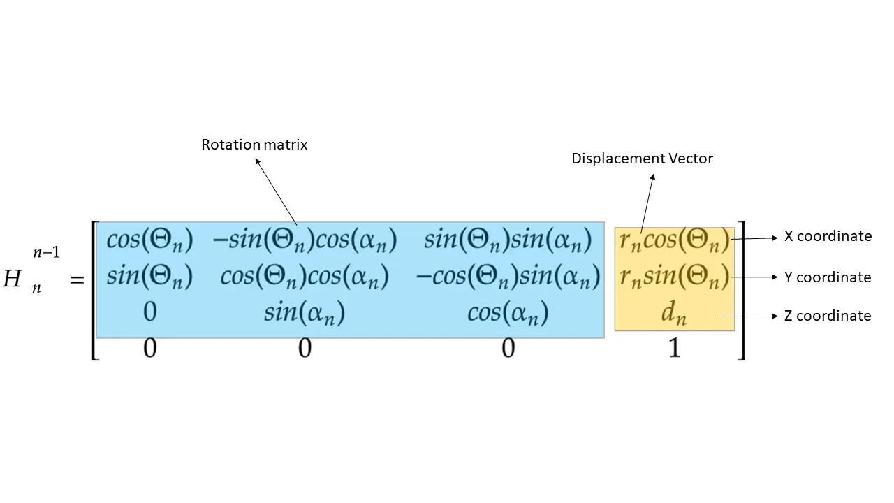

CODE EXPLANATION-

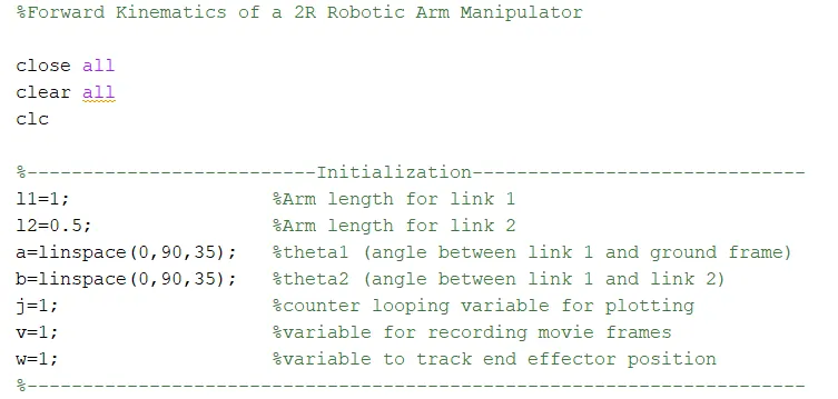
• Inputs are initialised for arm lengths and assigned to variables (“l1” &“l2”), arrays “a” & “b” for angles theta1 and theta2. Counter variables “v”, “w”, “j” for plotting, recording frames and getting.

• Two for loops are used, the first one varies `θ_1` values and similarly the second loop varies `θ_2`.

• User defined function forward_kinematics function is called in the script to compute the displacement vectors of the frames.

• The calculated positions of the displacement vectors are extracted from the 4x4 Homogenous Transformation matrix and then stored in temporary variables “q,t,w,s,e,m,n” using the counter looping variable “j”.

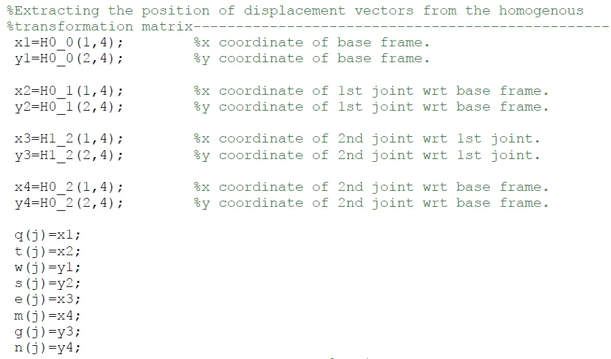
• Now the graph is plotted and each frame is stored in “N” in the same manner as done above for trigonometric method.

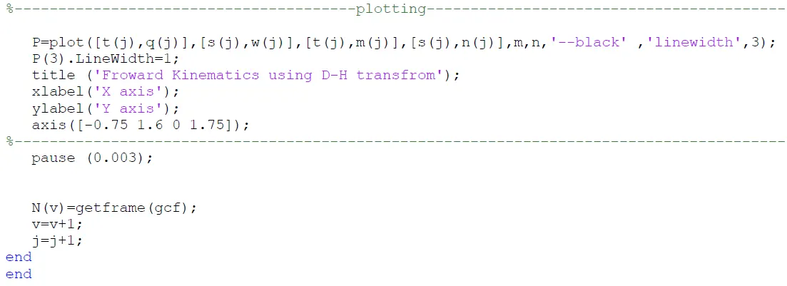
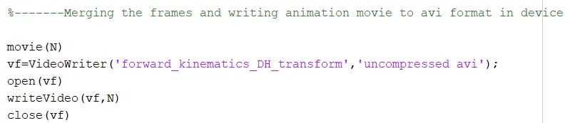
• After all this video for the animation is generated and stored in the drive.

• VideoWriter function generates an empty video in the .avi format and is stored in a variable “vf”.

• Open command opens the empty video file generated by VideoWriter, then writeVideo function writes the frames stored in the array “N" into the video file, close command closes the videofile

Function forward_kinematics explanation-

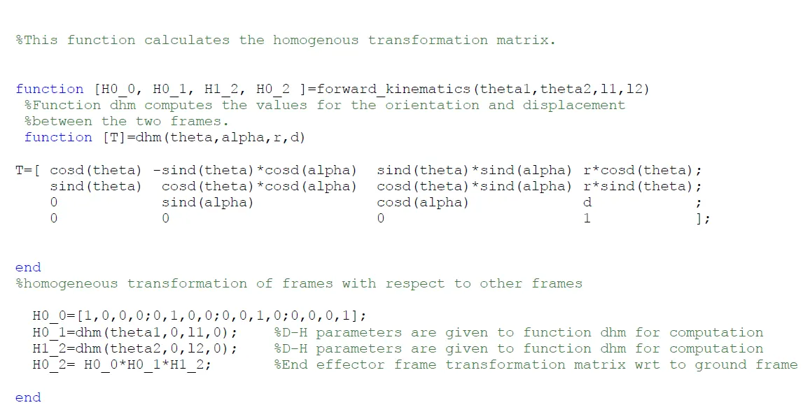
The function forward_kinematics is used for the computation of Homogeneous Transformation Matrix to find out the position and orientation of end effector. Details about the Homogenous Transformation matrix has been explained above.

This function returns four outputs-“H0_0, H0_1, H1_2, H0_2” and takes four inputs as well.

• H0_0 is the transformation of base frame wrt base frame.
• H0_1 is the transformation of 1^st frame wrt base frame.
• H1_2 is the transformation of 2^nd frame wrt 1^st
• H0_2 is the transformation of 2^nd frame wrt base frame.

Here we have a sub-function “dhm” that takes D-H parameters as inputs and returns calculated homogeneous transformation matrix

MATLAB Script-

%Forward Kinematics of a 2R Robotic Arm Manipulator

close all
clear all
clc

%--------------------------Initialization------------------------------
l1=1;                  %Arm length for link 1
l2=0.5;                %Arm length for link 2
a=linspace(0,90,35);   %theta1 (angle between link 1 and ground frame)
b=linspace(0,90,35);   %theta2 (angle between link 1 and link 2)
j=1;                   %counter looping variable for plotting
v=1;                   %variable for recording movie frames
w=1;                   %variable to track end effector position
%----------------------------------------------------------------------
%Using Denavit-Hartenberg Homogenous Transfrom for finding the end-effector
%position

for i=1:length(a)
    
for k=1:length(b)
      
    
   [H0_0,H0_1,H1_2,H0_2]=forward_kinematics(a(i),b(k),l1,l2);  %call to the user made function "forward_kinematics.m"
   
   %Extracting the position of displacement vectors from the homogenous
   %transformation matrix--------------------------------------------------
    x1=H0_0(1,4);        %x coordinate of base frame.
    y1=H0_0(2,4);        %y coordinate of base frame.
    
    x2=H0_1(1,4);        %x coordinate of 1st joint wrt base frame.
    y2=H0_1(2,4);        %y coordinate of 1st joint wrt base frame.
    
    x3=H1_2(1,4);        %x coordinate of 2nd joint wrt 1st joint.
    y3=H1_2(2,4);        %y coordinate of 2nd joint wrt 1st joint.
    
    x4=H0_2(1,4);        %x coordinate of 2nd joint wrt base frame.
    y4=H0_2(2,4);        %y coordinate of 2nd joint wrt base frame.
    
    q(j)=x1;
    t(j)=x2;
    w(j)=y1;
    s(j)=y2;
    e(j)=x3;
    m(j)=x4;
    g(j)=y3;
    n(j)=y4;
%---------------------------------------plotting------------------------------------------------------------
 
   P=plot([t(j),q(j)],[s(j),w(j)],[t(j),m(j)],[s(j),n(j)],m,n,'--black' ,'linewidth',3);
   P(3).LineWidth=1;
   title ('Froward Kinematics using D-H transfrom');
   xlabel('X axis');
   ylabel('Y axis');
   axis([-0.75 1.6 0 1.75]);
%-------------------------------------------------------------------------------------------------------------  
   pause (0.003);
  
   
   N(v)=getframe(gcf);
   v=v+1;
   j=j+1;
end
end

%-------Merging the frames and writing animation movie to avi format in device

movie(N)
vf=VideoWriter('forward_kinematics_DH_transform','uncompressed avi');
open(vf)
writeVideo(vf,N)
close(vf)

Function forward_kinematics script-

%This function calculates the homogenous transformation matrix.

function [H0_0, H0_1, H1_2, H0_2 ]=forward_kinematics(theta1,theta2,l1,l2)
 %Function dhm computes the values for the orientation and displacement
 %between the two frames.
 function [T]=dhm(theta,alpha,r,d)

T=[ cosd(theta) -sind(theta)*cosd(alpha)  sind(theta)*sind(alpha) r*cosd(theta);
    sind(theta)  cosd(theta)*cosd(alpha)  cosd(theta)*sind(alpha) r*sind(theta);
    0            sind(alpha)              cosd(alpha)             d            ;
    0            0                        0                       1            ];   


end
%homogeneous transformation of frames with respect to other frames

  H0_0=[1,0,0,0;0,1,0,0;0,0,1,0;0,0,0,1]; 
  H0_1=dhm(theta1,0,l1,0);    %D-H parameters are given to function dhm for computation
  H1_2=dhm(theta2,0,l2,0);    %D-H parameters are given to function dhm for computation
  H0_2= H0_0*H0_1*H1_2;       %End effector frame transformation matrix wrt to ground frame
  
end

Errors encountered while coding-

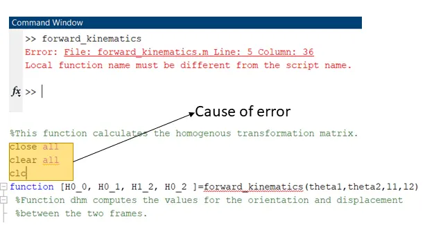
For implementing function in MatLab script files the script name and function name must be same so to rectify this error clear all, close all, clc were removed from the code.

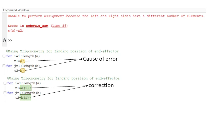
This error occurred because only one value for theta1 (a) and theta2 (b) was available and no loop counter variable was used.

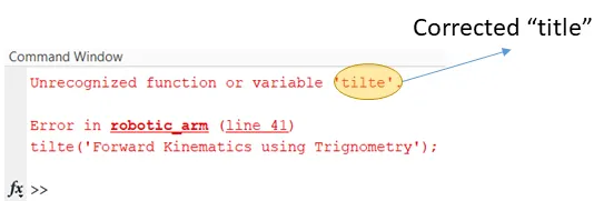
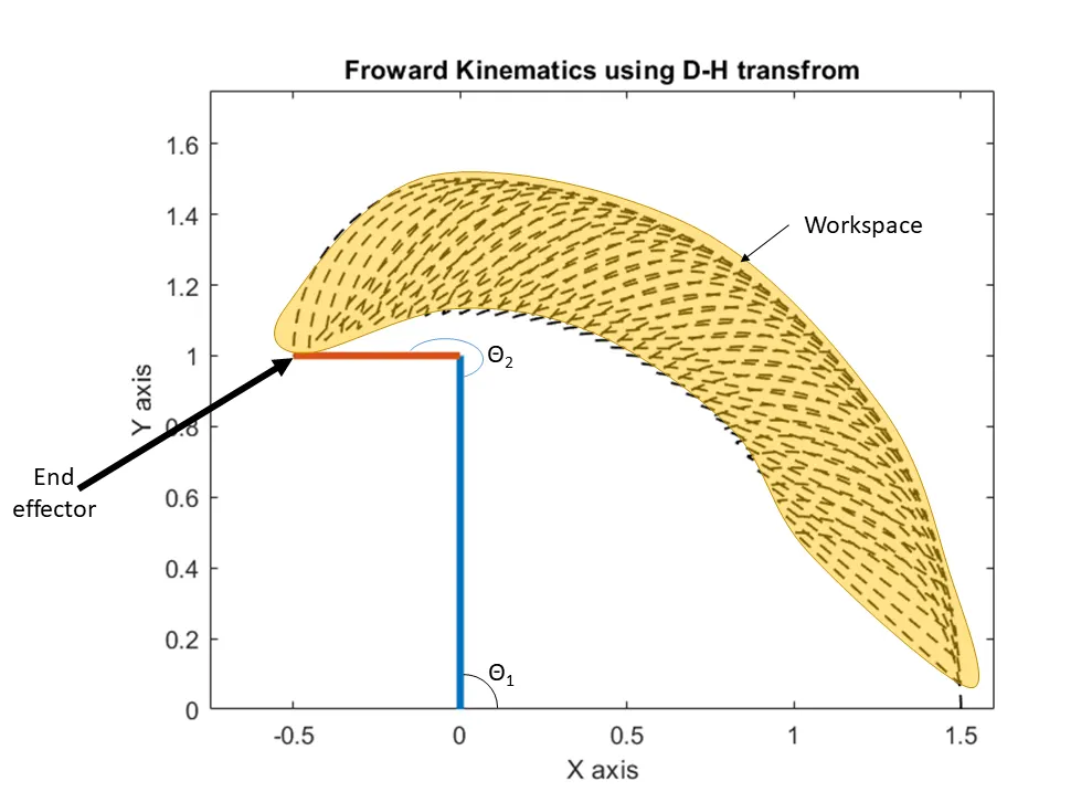
OUTPUT-

D-H transform Simulation Video

Results and Conclusion-

In today’s world we are surrounded by robots in all the fields be it science exploration, industrial setups or even in medical treatments procedures as well. With the advent of Industrial revolution 4.0 the industries are now shifting towards automation that is purely possible because of robotic manipulators.

A robotic manipulator can work for numerous hours doing intricate detailed work without getting tired, some notable examples of robotic manipulators include articulated manipulator for welding and painting processes, SCARA manipulators for pick and place operations, parallel manipulators like Steward-Gough platform for aircraft simulation and much more.

To make all these stuff work, studying the kinematics of the manipulator is necessary. Here, were successfully simulated a 2-DOF manipulator with revolute joints with the help of Denavit-Hartenberg transformation in MATLAB.

References-

Robotics by Angela Sodemann

S K Saha - Introduction To Robotics- MC GRAW HILL INDIA