Aim-Calculation of Thermal Efficiency of (Mazda MX-5 Miata) and plotting the P-V curve for it.

Objectives-

• To find the state variables at various state points using thermodynamic relations.
• To find the volume trace of combustion chamber during compression and expansion stroke.
• To calculate the thermal efficiency of the engine and plot the data to get Property change (P-V) diagram.
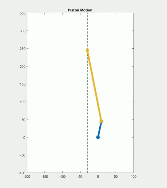
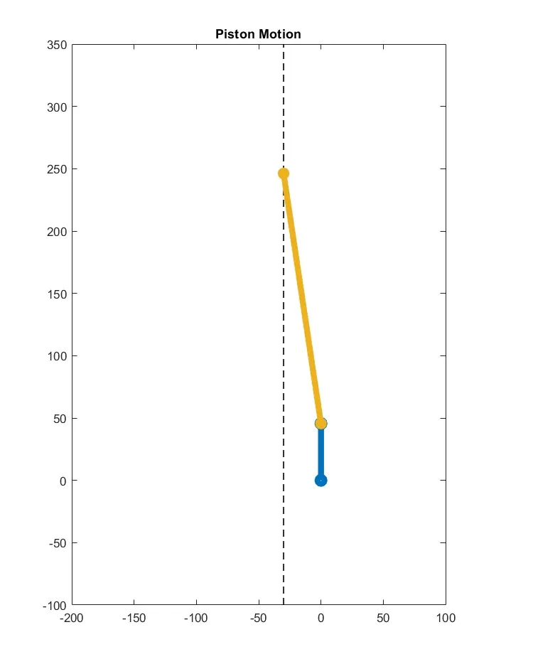
• To simulate the piston kinematics on screen.

Introduction-

We cannot imagine the world without Cars, Bikes, and Airplanes or in fact without the automotive and aviation industry. All these entities are based on thermodynamics. Talking about reciprocating engines where the piston reciprocates up and down and transmits power through the help of connecting rod and slider mechanism to the final drivetrain in vehicles.

A vast majority of reciprocating engines today are based on four-stroke cycle, which comprises four-strokes or two-revolutions of crankshaft. The under lying principle petrol engines (SI ENGINES) whether it being two or four stroke remains the same i.e. Otto’s cycle named after its inventor Nicolaus Otto. Otto cycle is a thermodynamic property change cycle that gives us the description of change in mass of gas when it is subjected to change in pressure, volume and temperature.

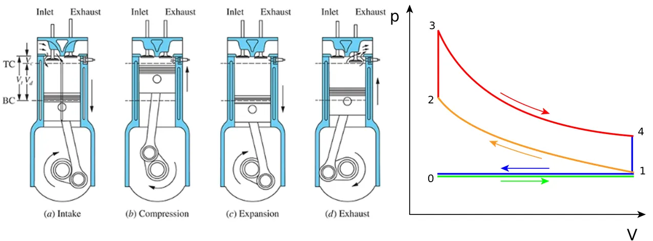
In the above, figure a four-stroke SI engine alongside with the ideal Otto cycle diagram where the Otto cycle’s processes are in sync with piston kinematics of the engine.

The processes are as follows-

• INTAKE (0-1)
• COMPRESSION (1-2)
• SPARK PLUG IGNITION (2-3)
• EXPANSION (3-4)
• EXHAUST (1-0)

The PV diagram models relationship among Pressure and Volume for an ideal gas (which have no interactions and its molecules occupy negligible space). The PV diagram for ideal Otto cycle consists-

• Two isochoric process
• Two adiabatic process
• Two isobaric process

Process 0 to 1-

This is the Intake process where the piston moves from TDC to BDC and charge (air-fuel mixture) comes inside the chamber without any change in pressure (isobaric process).

Process 1 to 2-

In this process the piston moves from BDC to TDC thereby compressing the charge and increasing the pressure and temperature however no heat exchange occurs (adiabatic process).

Process 2 to 3-

During the process the spark plug ignites and heat addition takes place at constant volume (isochoric process) and huge amount of energy gets generated.

Process 3 to 4-

The energy that was generated in the previous steps pushes the piston toward BDC thereby increasing the volume, this is referred as power stroke (adiabatic process).

Process 4 to 1 and 0 to 1-

After the power stroke the piston moves to TDC by the virtue of inertia of flywheel, all the waste gases starts getting removed from the chamber during which the games molecules loses some kinetic energy thereby reducing pressure (4 to 1), then the exhaust stroke (0 to 1) occurs and all the residual waste gets expelled without changing the pressure.

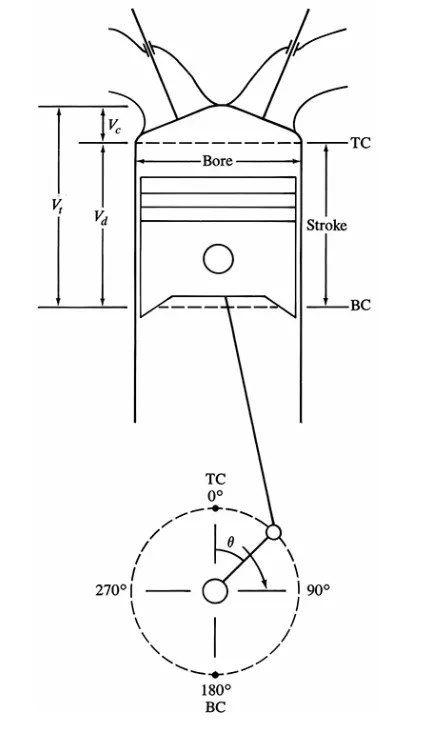
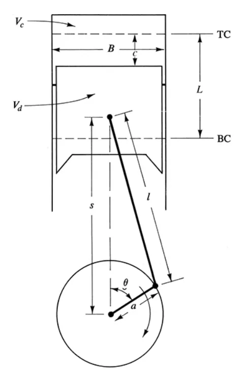
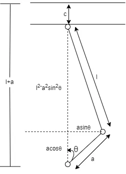
Geometrical Relations of Reciprocating Engines-

Here,

`θ = "crank radius"`

`B = "bore"`

`L = "stroke"`

`l = "length of connecting rod"`

`a = "crank radius"`

`c = "piston clearance from TDC"`

`C _r = ("maximum cylinder volume")/(" minimum cylinder volume ")= (V _d + V _c )/V _c`

`V _d = "swept volume"`

`V_ c = "clearance volume "= V _d /(C _r − 1)`

`a = "crank radius" = L /2`

`R = "connecting rod "/"crank radius" = l /a`

`"The cylinder volume V at any crank angle is given as : "V = V _c + V _d`

Using geometrical relations ‘c’ can be written as –

(‘c’ gives the instantaneous piston position at any crank angle)

`c=l+a-[(l^2-a^2 sin^2 θ)^(1⁄2)+acosθ]`

`c=L/2[R+1-cosθ-(R^2-sin^2 θ)^(1⁄2)]`

Cylinder volume at any crank angle is

`V=V_c+π/4 B^2 c`

`V=V_c+π/4 B^2 {L/2 [R+1-cosθ-(R^2-sin^2 θ)^(1⁄2) ]+L}`

`V=V_c+V_d {1/2 [R+1-cosθ-(R^2-sin^2 θ)^(1⁄2) ]+1}`

`V=V_c+V_c (c_r-1){1/2 [R+1-cosθ-(R^2-sin^2 θ)^(1⁄2) ]+1}`

`V/V_c =1+(c_r-1){1/2 [R+1-cosθ-(R^2-sin^2 θ)^(1⁄2) ]+1}`

Position analysis of Piston –

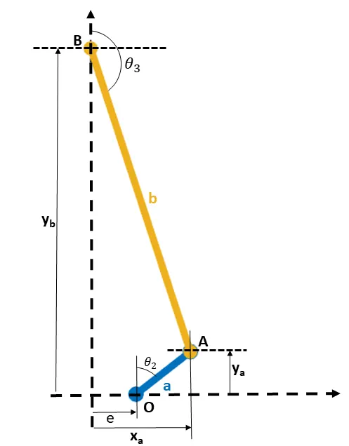
We have crank angle `theta_2` as the input and we intend to find the position and orientation of piston (‘B’) and `theta_3`.

`x_a=e+a sin⁡ θ_2`

`y_a=a cos⁡θ_2`

From the figure, we obtain

`e+a sin⁡θ_2=b sin⁡θ_3`

`sin⁡θ_3=1/b (e+a sin⁡θ_2 )`

`y_b=a cos⁡θ_2-b cos⁡θ_3`

`cos⁡θ_3 =-1/b sqrt(b^2-(e+a sin⁡θ_2 )^2 )`

Here negative sign indicates obtuse angle for `theta_3`

Thermodynamic relations for the processes-

Assumptions-

• Temperature after combustion (T₃) = 2300^o C
• Pressure at state point 1 (P₁) = 101325 N/m²
• Temperature at state point 1(T₁) = 500 ^o C

Engine parameters of Mazda MX-5 Miata-

• Bore = 0.0835m
• Stroke = 0.0912m
• Compression ratio (`C_r`) = 13:1
• Connecting rod length = 0.20064m

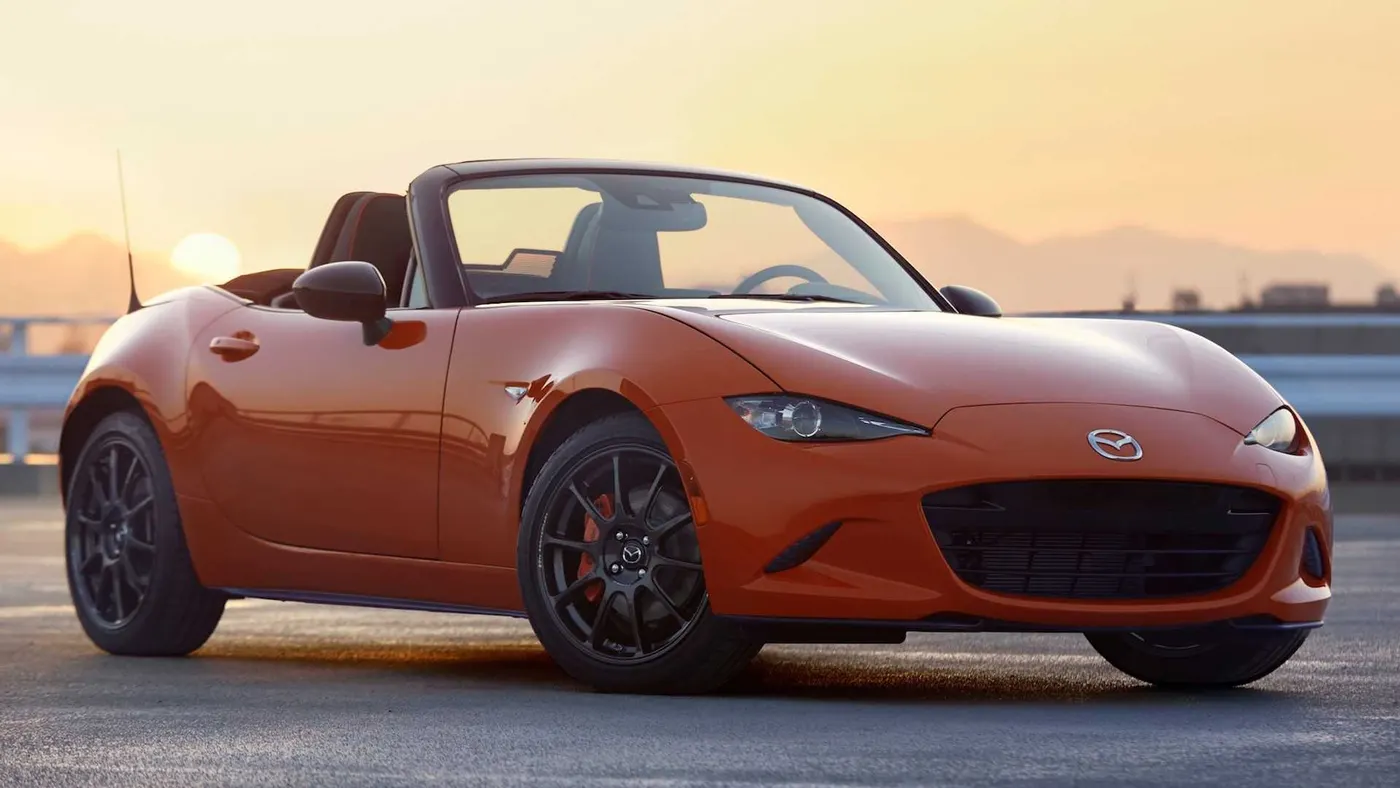
Mazda MX-5 Miata Specifications...

State Variables-

POINT 1-

`P_1="101325 "N//m^2`

`V_1=V_c+V_d`

`T_1="2300"^oC`

POINT 2-

`"For isentropic compression "(PV^γ="constant")`

`P_2 V_2^γ=P_1 V_1^γ`

`P_2=P_1 (V_1^γ/V_2^γ )`

`P_2=P_1 (c_r )^γ`

`V_2=V_c`

`T_2=(P_2 V_2 T_2)/(P_1 V_1 )`

POINT 3-

`P_3=P_2 (T_3/T_2 )`

`V_3=V_2`

`T_3=(P_3 V_3 T_2)/(P_2 V_2 )`

POINT 4-

`P_4=P_3 (V_3/V_4 )^γ`

`V_3=V_2`

`T_4=(P_4 V_4 T_3)/(P_3 V_3 )`

Thermal efficiency-

`η_(th)=1-(T_4-T_1)/(T_3-T_2 )`

CODE EXPLANATION-

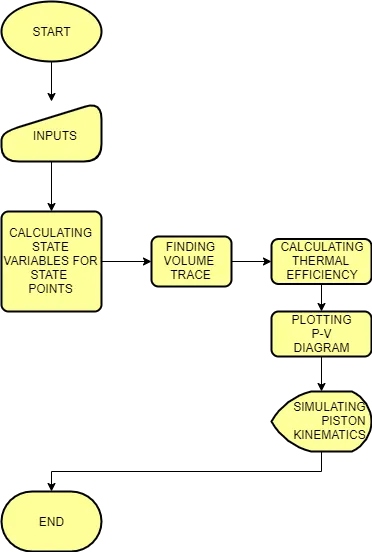
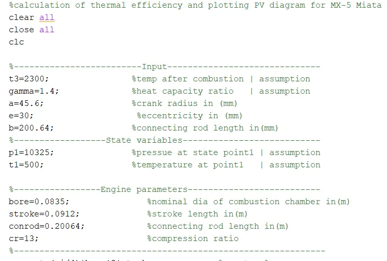
• Inputs are initialised with relevant assumptions, state variables for state point 1 were assumed and initialised, and engine parameters of Mazda MX-5 Miata were initialised.

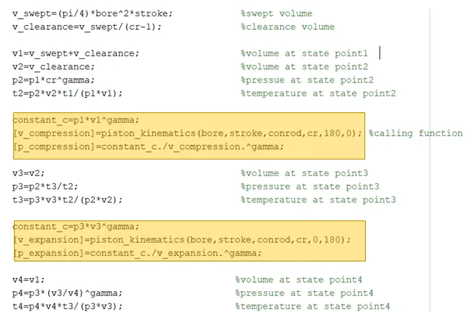
• Calculating the value for state variables at different state points during the thermodynamic cycle with the help of relations and formulas explained above. A user defined function ‘piston_kinematics’ was called to find the volume trace as the pressure and volume change.

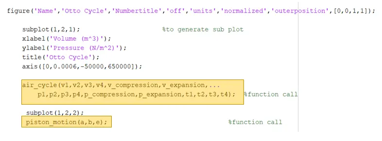
• A figure window is being created named ‘Otto Cycle’ with its number title off and window’s appearance was altered, measurement units were normalised where the lower-left corner of the container maps to (0,0) and the upper-right corner maps to (1,1) thus the position of figure window was set to [0,0,1,1] to get a full-screen figure window.
• The figure is divided into two parts using subplot one partition for plotting PV diagram and the other one for simulating piston motion.
• Labels, title and axes for the graph was adjusted.
• A call to the user defined function ‘air_cycle’ for plotting the PV diagram and calculating thermal efficiency.
• Next call was made to the ‘piston_motion’ function for simulating piston kinematics.

Function (piston_kinematics)-

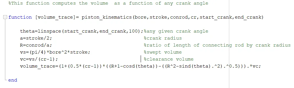
• This function computes volume inside combustion chamber at each given angle of the crankshaft, details about this have been explained above in theory section.
• It takes inputs arguments as – bore, stroke, conrod, cr, start_crank, end_crank and returns output as volume_trace.

Function (air_cycle)-

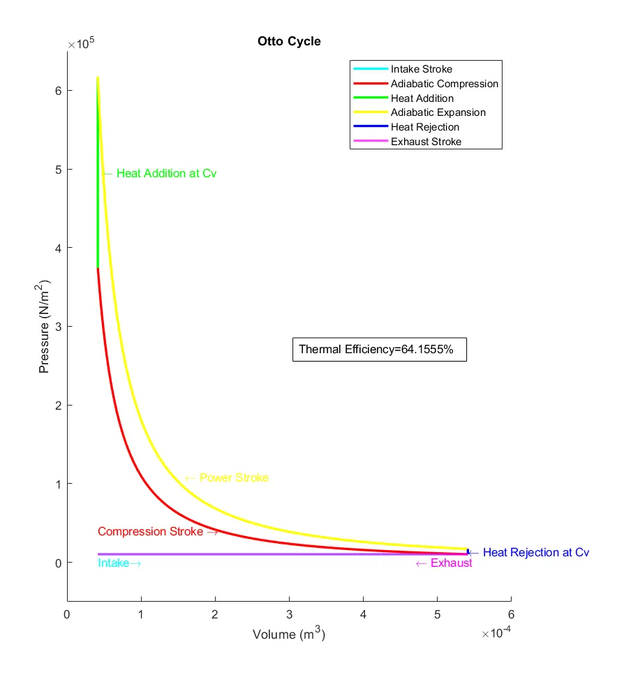
• Function air_cycle takes inputs arguments as volume, pressure and temperature of different state points and gives the output as shown below in the video.

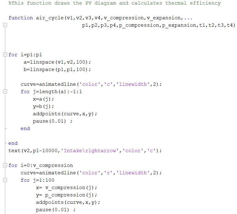
• To animate the intake process represented by cyan colour in the above video was done in the fashion explained below-

As already discussed intake is an isobaric process i.e. P1 doesn’t change and volume at TDC to BDC was changed from v2 to v1 respectively.

Two for loop were used one for generating linearly spaced vectors using linspace between v1, v2, p1 and stored in variables ‘a’ & ‘b’

To create animation ‘animatedline’ was used, line properties were defined i.e. colour and linewidth, animatedline object was also created using a local variable named ‘curve’.

Now the next loop comes to action, this loop was assigned the task to add data points to the object ‘curve’ using addpoints function and display each instance on screen by using pause.

After the looping text has been used to display the process name on the screen.

• Similarly all the remaining processes were animated using the same methodology.
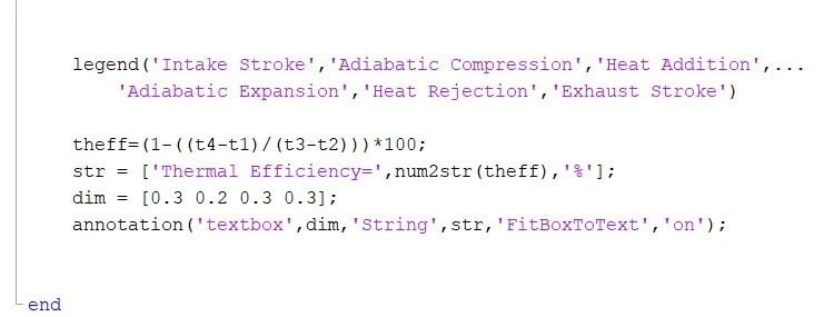
• After successful animation of respective curves legends were assigned.
• Next thermal efficiency was calculated using the thermodynamic relations and it value was assigned to variable ‘theff’.
• A string array was created with ‘Thermal efficiency’ as input array and num2str function was used to display the numerical value of thermal efficiency on the plot.
• To create text box on the plot annotation function was used.
• dim signifies the size and location specified as a four-element vector of the form [x y w h]. The first two elements specify the coordinates of the lower left corner of the text box and the second two elements specify the width and height of the annotation, respectively.

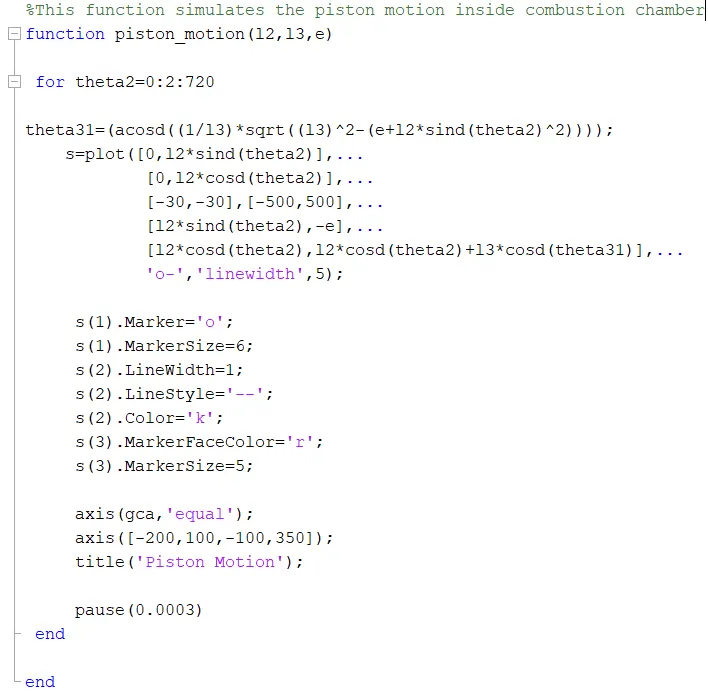
Function (piston_motion)-

• For simulating piston motion this was used wherein theta2 represents crank angle and theta31 represents orientation of the piston, this has been dealt in detail in introduction section.
• For the coding part links were plotted using plot function and an object [s] was created to alter the plot properties.
• Current axes for this subplot was set using gca command and axis style was set to equal (axis equal sets the aspect ratio so that the data units are the same in every direction). Now the axis was calibrated and title was given to the plot followed by pause to see the animation on screen.

MATLAB SCRIPT-

Main Script-

%calculation of thermal efficiency and plotting PV diagram for MX-5 Miata
clear all 
close all
clc 

%-------------------------Input------------------------------
t3=2300;                %temp after combustion | assumption
gamma=1.4;              %heat capacity ratio   | assumption
a=45.6;                 %crank radius in (mm)
e=30;                    %eccentricity in (mm)
b=200.64;               %connecting rod length in(mm) 
%------------------State variables---------------------------
p1=10325;               %pressue at state point1 | assumption
t1=500;                 %temperature at point1   | assumption

%-----------------Engine parameters--------------------------
bore=0.0835;               %nominal dia of combustion chamber in(m)
stroke=0.0912;             %stroke length in(m)
conrod=0.20064;            %connecting rod length in(m)    
cr=13;                     %compression ratio
%-------------------------------------------------------------
v_swept=(pi/4)*bore^2*stroke;            %swept volume
v_clearance=v_swept/(cr-1);              %clearance volume

v1=v_swept+v_clearance;                  %volume at state point1  
v2=v_clearance;                          %volume at state point2   
p2=p1*cr^gamma;                          %pressue at state point2   
t2=p2*v2*t1/(p1*v1);                     %temperature at state point2   

constant_c=p1*v1^gamma;                  
[v_compression]=piston_kinematics(bore,stroke,conrod,cr,180,0); %calling function
[p_compression]=constant_c./v_compression.^gamma;

v3=v2;                                   %volume at state point3  
p3=p2*t3/t2;                             %pressure at state point3  
t3=p3*v3*t2/(p2*v2);                     %temperature at state point3  

constant_c=p3*v3^gamma;
[v_expansion]=piston_kinematics(bore,stroke,conrod,cr,0,180);
[p_expansion]=constant_c./v_expansion.^gamma;

v4=v1;                                  %volume at state point4
p4=p3*(v3/v4)^gamma;                    %pressure at state point4 
t4=p4*v4*t3/(p3*v3);                    %temperature at state point4

figure('Name','Otto Cycle','Numbertitle','off','units','normalized','outerposition',[0,0,1,1]);
   
    s1=subplot(1,2,1);                     %to generate sub plot
    xlabel('Volume (m^3)');
    ylabel('Pressure (N/m^2)');
    title('Otto Cycle');
    axis([0,0.0006,-50000,650000]);

    
    air_cycle(v1,v2,v3,v4,v_compression,v_expansion,...
        p1,p2,p3,p4,p_compression,p_expansion,t1,t2,t3,t4);  %function call
     
    s=subplot(1,2,2); 
    piston_motion(a,b,e);                                    %function call
    

Function piston_kinematics-

%This function computes the volume  as a function of any crank angle 

function [volume_trace]= piston_kinematics(bore,stroke,conrod,cr,start_crank,end_crank)
   
    theta=linspace(start_crank,end_crank,100);%any given crank angle
    a=stroke/2;                               %crank radius
    R=conrod/a;                               %ratio of length of connecting rod by crank radius
    vs=(pi/4)*bore^2*stroke;                  %swept volume
    vc=vs/(cr-1);                             %clearance volume
    volume_trace=(1+(0.5*(cr-1))*((R+1-cosd(theta))-((R^2-sind(theta).^2).^0.5))).*vc;
    
end

Function air_cycle-

%This function draws the PV diagram and calculates thermal efficiency

function air_cycle(v1,v2,v3,v4,v_compression,v_expansion,...
                        p1,p2,p3,p4,p_compression,p_expansion,t1,t2,t3,t4)
   
    
    
for i=p1:p1
     a=linspace(v1,v2,100);
     b=linspace(p1,p1,100);
     
    curve=animatedline('color','c','linewidth',2);
    for j=length(a):-1:1
        x=a(j);
        y=b(j);
        addpoints(curve,x,y);
        pause(0.01) ;  
    end
  
end
text(v2,p1-10000,'Intakerightarrow','color','c');

for i=0:v_compression
    curve=animatedline('color','r','linewidth',2);
    for j=1:100
         x= v_compression(j);
         y= p_compression(j);
         addpoints(curve,x,y);
         pause(0.01) ;  
    end
  
end
text(v_compression(100),p_compression(65),'Compression Stroke rightarrow','color','r')
 for j=v2:v3
      a=linspace(v2,v3,100);
      b=linspace(p2,p3,100);
     curve=animatedline('color','g','linewidth',2);
    for j=1:length(a)
        x=a(j);
        y=b(j);
        addpoints(curve,x,y);
        pause(0.01) ;
    end
   
end
text(v3+0.000005,((p2+p3)/2),'leftarrow Heat Addition at Cv','color','g')

for j=0:v_expansion
     curve=animatedline('color','y','linewidth',2);
    for j=1:100
        x= v_expansion(j);
        y= p_expansion(j);
        addpoints(curve,x,y);
        pause(0.01) ;
    end
   
end
text(v_expansion(30),p_expansion(28),'leftarrow Power Stroke','color','y')
for j=v4:v1
      a=linspace(v4,v1,100);
      b=linspace(p4,p1,100);
      curve=animatedline('color','b','linewidth',2);
   for j=1:length(a)
        x= a(j);
        y= b(j);
        addpoints(curve,x,y);
        pause(0.01) ;
   end
  
end
    text((v1),((p1+p4)/2),'leftarrow Heat Rejection at Cv ','color','b') 
for i=p1:p1
     a=linspace(v1,v2,100);
     b=linspace(p1,p1,100);
     curve=animatedline('color',[1,0,1,0.7],'linewidth',2);
    for j=1:length(a)
        x=a(j);
        y=b(j);
        addpoints(curve,x,y);
        pause(0.01) ;  
    end
  
end
text(a(15),b(2)-10000,'leftarrow Exhaust','color','m');


    legend('Intake Stroke','Adiabatic Compression','Heat Addition',...
        'Adiabatic Expansion','Heat Rejection','Exhaust Stroke')
    
    theff=(1-((t4-t1)/(t3-t2)))*100;
    str = ['Thermal Efficiency=',num2str(theff),'%'];
    dim = [0.3 0.2 0.3 0.3];
    annotation('textbox',dim,'String',str,'FitBoxToText','on');
    
   
end

Function piston_motion-

%This function simulates the piston motion inside combustion chamber
function piston_motion(l2,l3,e)
 
 for theta2=0:2:720
    
theta31=(acosd((1/l3)*sqrt((l3)^2-(e+l2*sind(theta2)^2))));
    s=plot([0,l2*sind(theta2)],...
            [0,l2*cosd(theta2)],...
            [-30,-30],[-500,500],...
            [l2*sind(theta2),-e],...
            [l2*cosd(theta2),l2*cosd(theta2)+l3*cosd(theta31)],...
            'o-','linewidth',5);
    
     s(1).Marker='o';
     s(1).MarkerSize=6;
     s(2).LineWidth=1;
     s(2).LineStyle='--';
     s(2).Color='k';
     s(3).MarkerFaceColor='r';
     s(3).MarkerSize=5;
    
     axis(gca,'equal');
     axis([-200,100,-100,350]);
     title('Piston Motion');
   
     pause(0.0003)
 end
 
end

OUTPUT-

Results-

The engine parameters of Mazda MX-5 Miata were analysed by the MATAB scripts and the thermal efficiency was found to be equal to 64.15 % approximately. Piston motion was simulated appropriately .

Conclusions-

The thermal efficiency has been successfully computed in MATLAB. From the results we can confidently say that more than 30% of energy gets wasted during the operation of the engines due to various frictional losses and other contributing losses.

There is a big room in this domain for improvement. Nowadays automotive companies are trying to tackle this problem along with making engines more fuel efficient, like running super lean mixtures and using Miller cycle engines rather than Otto cycle based for better fuel economy.

References-

• Theory of Machines and Mechanisms by John J. Uicker Jr., Gordon R. Pennock, Joseph E. Shigley
• Robert L. Norton Design of Machinery (McGraw-Hill)
• John B. Heywood - Internal Combustion Engine Fundamentals (McGraw-Hill Education)
• Mazda MX-5 Engine Specifications
• https://www.mazdausa.com/siteassets/pdf/owners-optimized/2019/mx-5-miata-st/2019_mazda_mx5_features_specs.pdf
• https://www.roadandtrack.com/new-cars/car-technology/a22713694/2019-mazda-mx-5-miata-engine-tech/