Perform Curve fitting using Linear Regression Analysis.
Aim- Perform Curve fitting using Linear Regression Analysis.
Objectives-
- To perform curve fitting using Least Square Regression
- To Validate the results using the Curve Fit TOOLBOX in MatLab
Introduction
Regression Analysis refers to the study of relationship between a dependent and one or more independent variables. This statistical technique can be used for modelling future relationships between the variables. When the relationship is approximated using a straight line it is called linear regression and when it is a curve it can be called as curvilinear regression or for even more complicated datasets it is non-linear regression.
Curve fitting is the process of constructing a curve, or mathematical function that has the best fit to a series of data points.
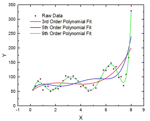
Curve fitting can be done in two ways-
- Least Square Regression- Here we have discrete values of data and we tend to derive a single curve that represents the general flow of the data.
- Interpolation- Whereas here we try to fit a curve or a series of curves that pass directly through each of the points.
However, In this project we will be using Least Square Regression.
Linear Curve Fitting (Linear Regression)-
The general form of a straight line is given by,
`ŷ=b_1x+b_0`
But when using this kind of model for any specific observation, the actual value can deviate from the predicted value. These deviation are called errors/residues.
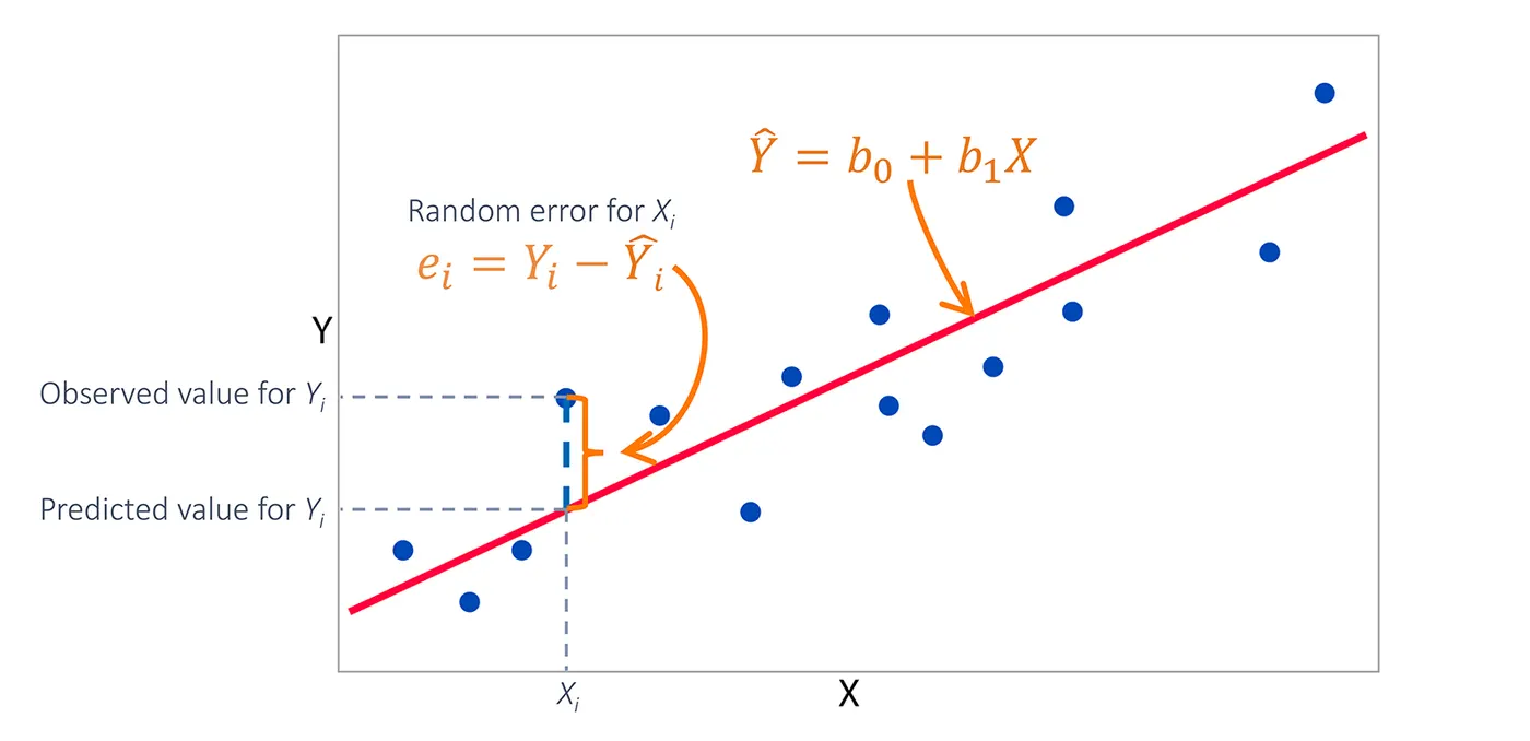
The better the line fits the data points the smaller the residuals get. Mathematical we can put it in this way
`∑(y_i−ŷ_i)^2=∑e_i^2`
Line with the smallest value of `∑(e_i)^2` is the best fit. This is the method of least squares where we find values of the intercept and slope coefficient that minimize the sum of the squared errors.
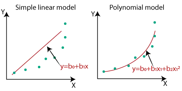
Polynomial Regression-
It is a regression analysis in which the relationship between the independent variable and the dependent variable is modelled as an nth degree polynomial in independent variable.
We can write a general polynomial as,
`y = b_0 + b_1 x + b_2 x ^2 + b_3 x^ 3 + ⋯ + b _n x ^n`
Measures of Regression Fit-
To know the answer to the question “How good is our regression fit?” we ought to understand measures of fit.
Coefficient of Determination (`R^2`)-
It explains how good the fit is in explaining the variation between the dependent and independent variables on a scale of 0-1. Mathematical we can pose it in this way
`R^2=1-(∑e_i^2 )/(∑(y_i-ȳ _i )^2 )`
`R^2=1-(SSR)/(SST)=(SST-SSE)/(SST)`
SSR is the sum of squared residuals, and is defined as-
`SSR=∑e_i^2`
The total sum of squares (SST) is the sum of squared deviations of the from their average. Thus we have
`SST=∑(y_i-ȳ _i )^2`
Sum of squares (SSE) is the sum of squared deviations of the predicted values `ŷ _i` , from the average of the `ȳ _i` .
`SSE=∑(ŷ_i-ȳ _i )^2`
Since `R^2` lies between 0 and 1. We can see that a perfect fit (no errors made), implies `R^2=1` and `SSR=0` . On the contrary, if our estimated regression line does not explain any variation then we have `SSE=0` and consequently `R^2=0` .
Adjusted `R^2`-
It is mainly R-Squared but it takes account of the number of predictors upon defined for the degrees of freedom. R² always increases as we add up variables to the model, even if they are not related as well. The adjusted-R² will increase only if the new variable will add some fair amount of variation.
`R_(adj)^2=1-[(1-R^2 )(n-1)/(n-k-1)]`
Where,
- n=number of data points
- k=number of independent variables
Standard Error of the Regression (SER)-
The Standard Error of the Regression is an estimator of the standard deviation of the residuals `(e_i ).`
`SER=sqrt(1/(n-2) ∑e_i^2 )`
Root Mean Squared Error (RMSE) –
It is the standard deviation of random component in the data and is defined as
`RMSE=sqrt((∑(ŷ _i-ȳ _i )^2 )/n)`
Lower values of RMSE indicate a better fit.
MATLAB Implementation using Programming-
Curve Fitting-
CODE EXPLANATION-
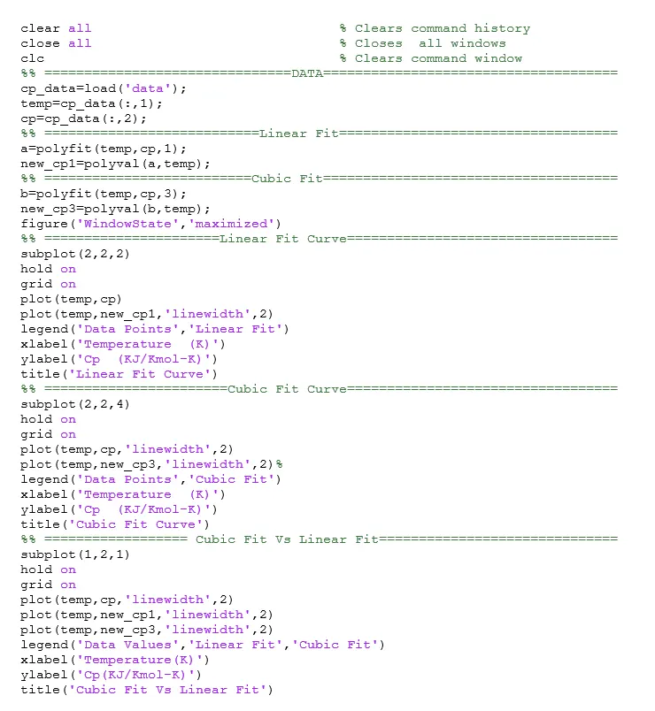
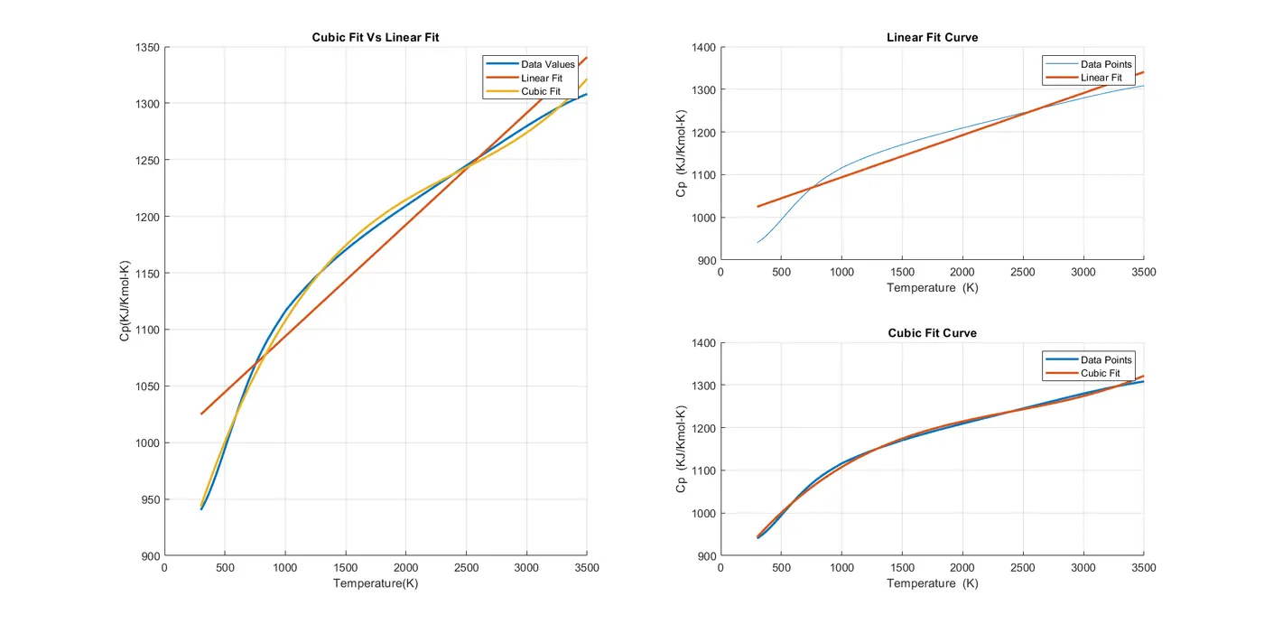
- First the data file was loaded from the local directory into a variable cp_data and its columns were assigned temp & cp, next computing the coefficients of the linear polynomial and storing the values in variable ‘a’, predicted points were calculated using the polyval function and then graphs were plotted. Similar fashion was followed for the cubic fit as well.
Output-
We can clearly see from the plots below that cubic fit is far better than a linear fit.
But this creates a problem, in the command window we can notice,

Badly conditioned means that the solution of the system of linear equations critically depends on rounding errors due to the limited precision. In order to solve this issue we can use
- Centering and Scaling
- Using Split wise regression
clear all                               % Clears command history
close all                               % Closes  all windows
clc                                     % Clears command window
%% ===============================DATA=====================================
cp_data=load('data');
temp=cp_data(:,1);
cp=cp_data(:,2);
%% ===========================Linear Fit===================================
a=polyfit(temp,cp,1);
new_cp1=polyval(a,temp);
%% ==========================Cubic Fit=====================================
b=polyfit(temp,cp,3);
new_cp3=polyval(b,temp);
figure('WindowState','maximized')
%% ======================Linear Fit Curve==================================
subplot(2,2,2)
hold on
grid on
plot(temp,cp)
plot(temp,new_cp1,'linewidth',2)
legend('Data Points','Linear Fit')
xlabel('Temperature  (K)')
ylabel('Cp  (KJ/Kmol-K)')
title('Linear Fit Curve')
%% =======================Cubic Fit Curve==================================
subplot(2,2,4)
hold on
grid on
plot(temp,cp,'linewidth',2)
plot(temp,new_cp3,'linewidth',2)%
legend('Data Points','Cubic Fit')
xlabel('Temperature  (K)')
ylabel('Cp  (KJ/Kmol-K)')
title('Cubic Fit Curve')
%% ================== Cubic Fit Vs Linear Fit==============================
subplot(1,2,1)
hold on
grid on
plot(temp,cp,'linewidth',2)
plot(temp,new_cp1,'linewidth',2)
plot(temp,new_cp3,'linewidth',2)
legend('Data Values','Linear Fit','Cubic Fit')
xlabel('Temperature(K)')
ylabel('Cp(KJ/Kmol-K)')
title('Cubic Fit Vs Linear Fit')
Curve Fitting with error estimates-
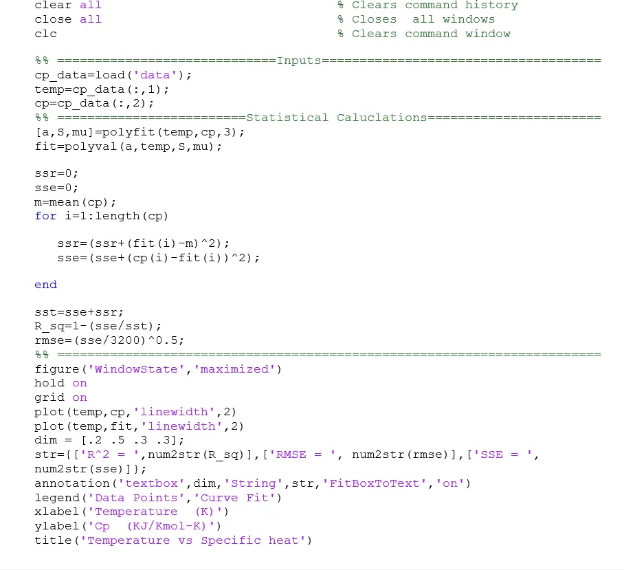
CODE EXPLANATION-
- Raw Data is being prepared to get analysed upon.
- Polyfit function is used to get cubic coefficients stored in ‘a’ ,a structure ‘S’ which will be used in polyval for error estimated and mu, which is a two-element vector with centering and scaling values. mu (1) is mean, and mu(2) is standard deviation. Using these values, polyfit centers temp at zero and scales it to have unit standard deviation.
- Polyval function is used for polynomial evaluation with error estimates, centered & scaled output, is stored in variable ‘fit’.
- Some statistical calculations are performed for finding SSR, SSE, RMSE, R_sq in order to evaluation goodness of the fit.
- Furthermore, data is plotted and the goodness parameters were displayed on the figure window as an annotation.
Output-
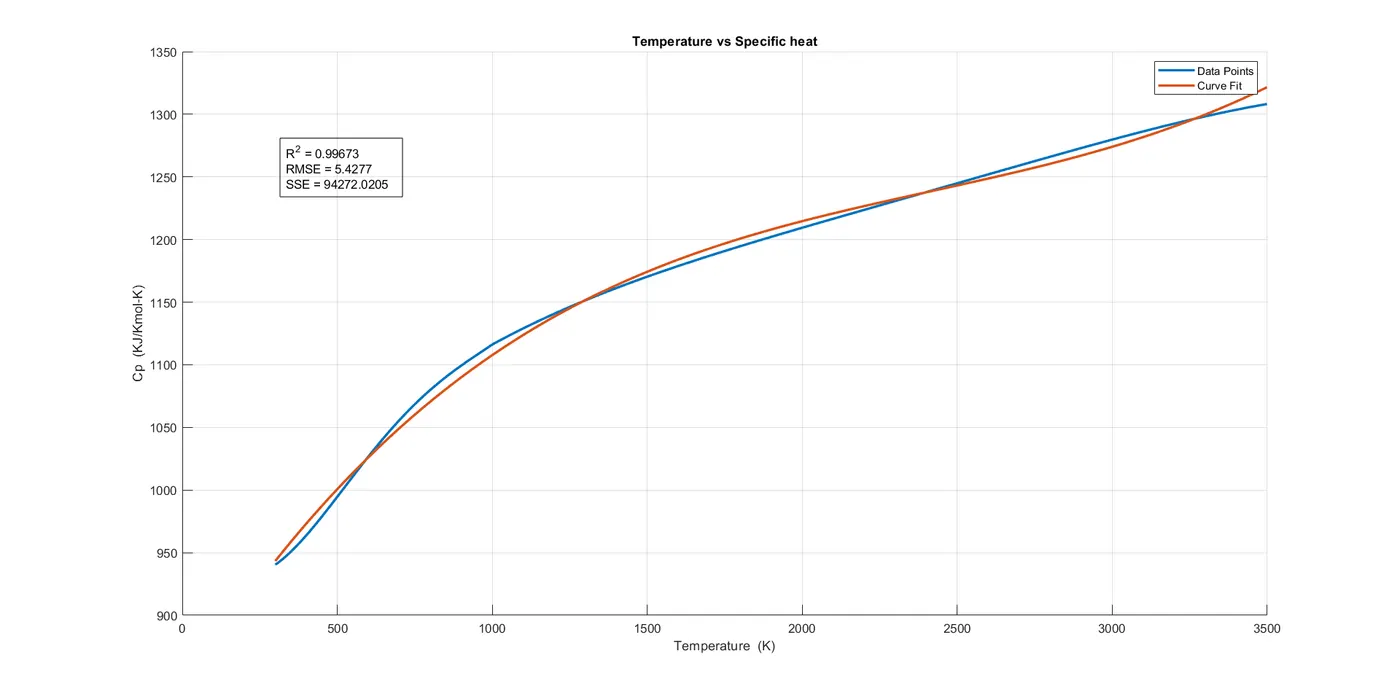
We get a cubic fit with error estimates and scaling with R2 of value 0.99673 showing a better fit.
clear all                               % Clears command history
close all                               % Closes  all windows
clc                                     % Clears command window

%% =============================Inputs=====================================
cp_data=load('data');
temp=cp_data(:,1);
cp=cp_data(:,2);
%% =========================Statistical Caluclations=======================
[a,S,mu]=polyfit(temp,cp,3);
fit=polyval(a,temp,S,mu);

ssr=0;
sse=0;
m=mean(cp);
for i=1:length(cp)

   ssr=(ssr+(fit(i)-m)^2);
   sse=(sse+(cp(i)-fit(i))^2);

end

sst=sse+ssr;
R_sq=1-(sse/sst);
rmse=(sse/3200)^0.5;
%% ========================================================================
figure('WindowState','maximized')
hold on
grid on
plot(temp,cp,'linewidth',2)
plot(temp,fit,'linewidth',2)
dim = [.2 .5 .3 .3];
str={['R^2 = ',num2str(R_sq)],['RMSE = ', num2str(rmse)],['SSE = ', num2str(sse)]};
annotation('textbox',dim,'String',str,'FitBoxToText','on')
legend('Data Points','Curve Fit')
xlabel('Temperature  (K)')
ylabel('Cp  (KJ/Kmol-K)')
title('Temperature vs Specific heat')
Curve Fitting with Stepwise Regression-
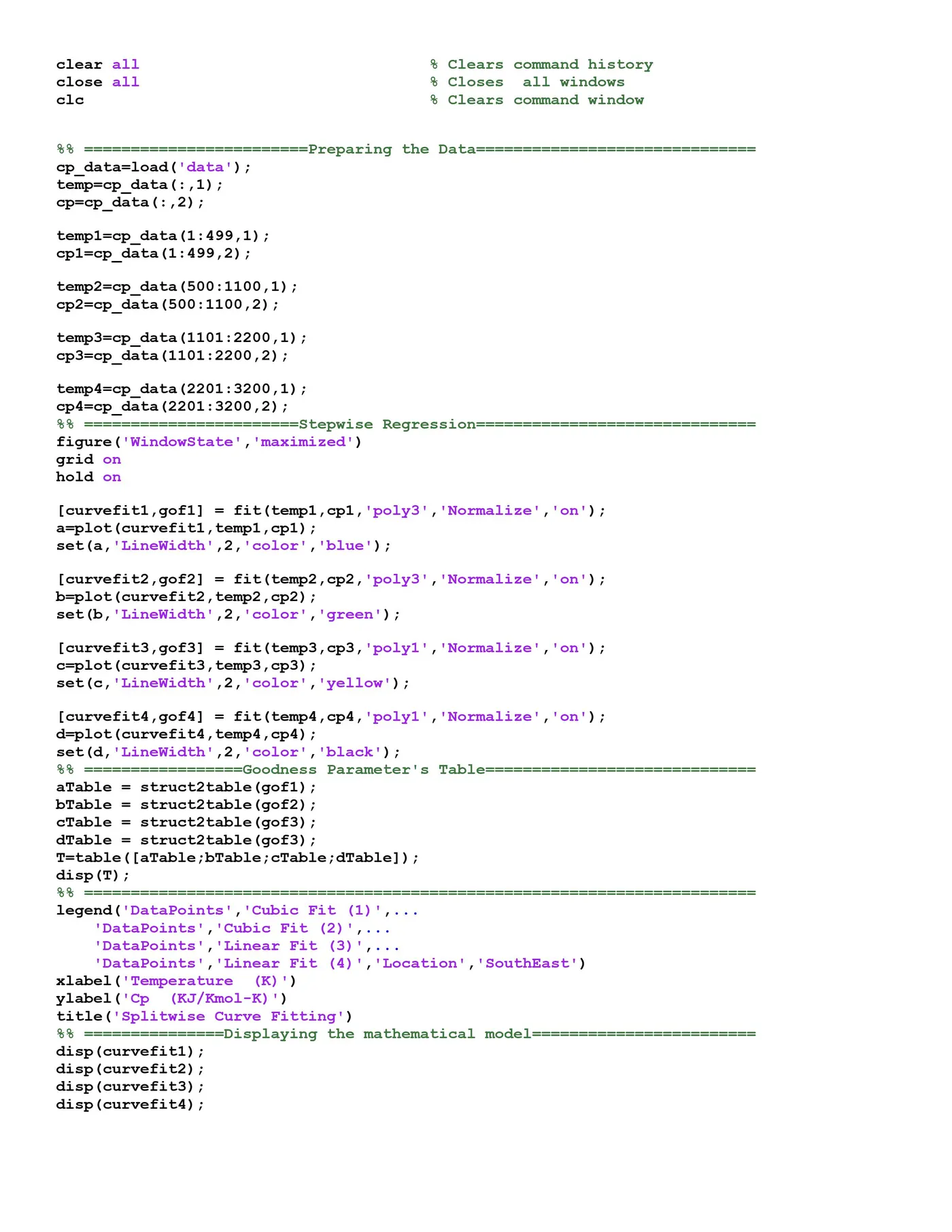
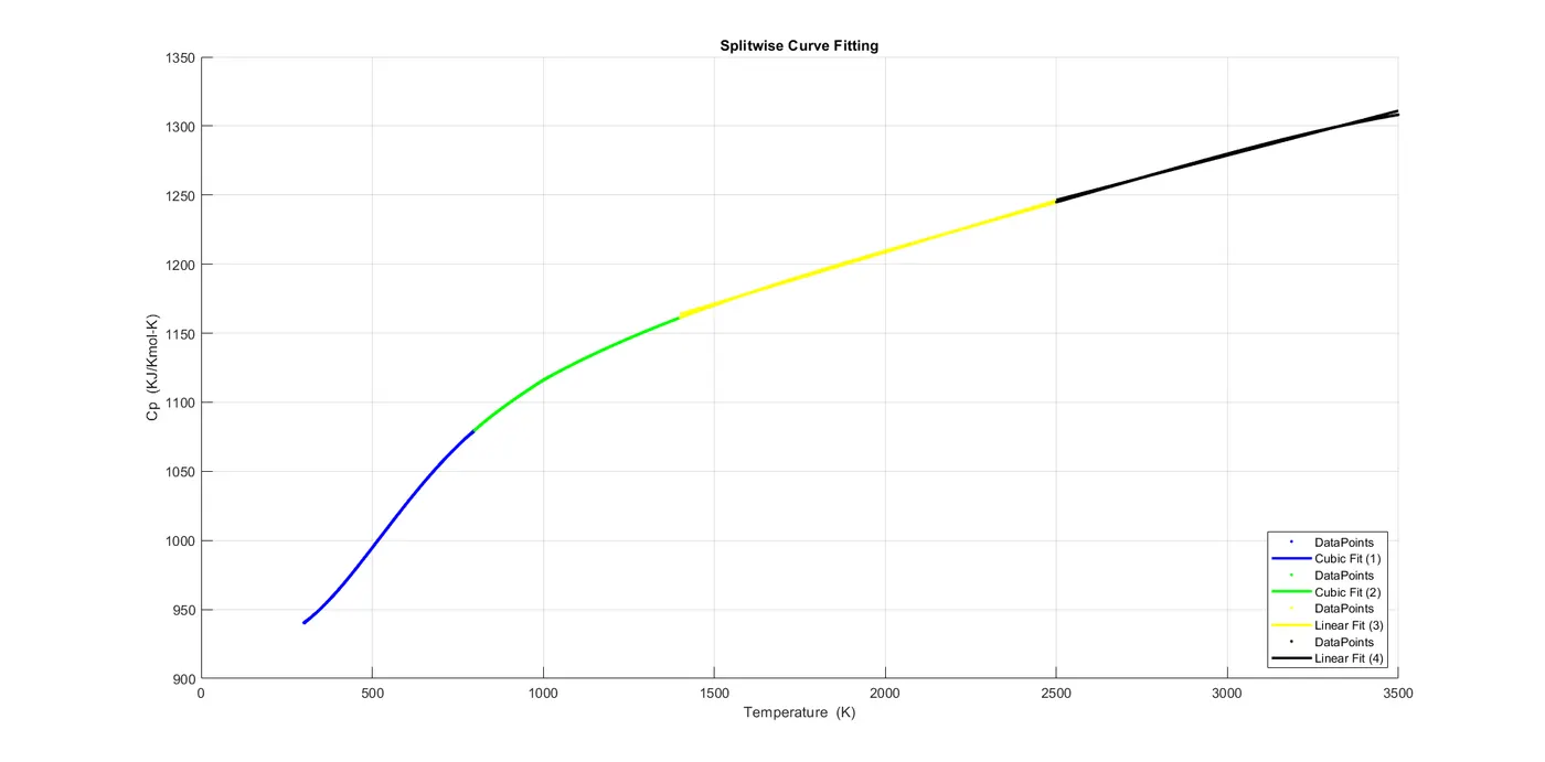
In this stepwise regression method the entire data set is split-up into four intervals with two cubic and two linear models for the fitting algorithm.
CODE EXPLANATION-
- Raw data is prepared or simply put it gets split up into four intervals with respective variables.
- Stepwise regression is used to fit the data points, fit function is used for this implementation wherein the output arguments are fit object and a structure containing goodness of fit statistics.
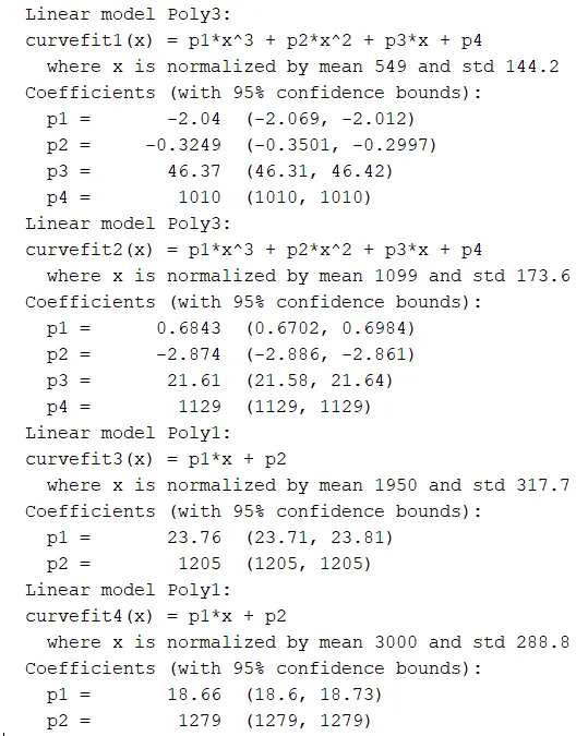
- A goodness of fit is constructed for the four intervals using the gof1, gof2, gof3, gof4
- Mathematical model thus generated is displayed on the command window.
Output-
Thus split wise method is successfully employed and we get the model as-
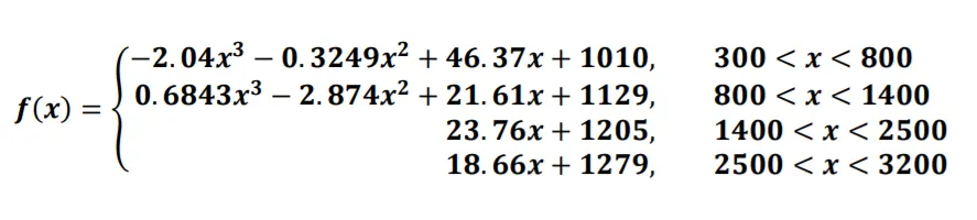
where,
- `x=Temperature`
- `f(x)="Specific Heat "(C_p)`
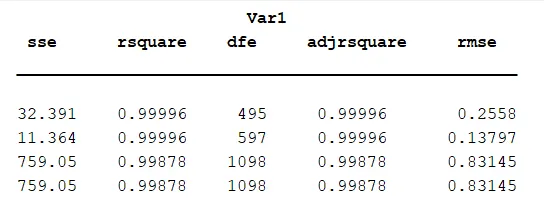
From the table given below we can clearly infer by looking at the R square value that it is a good fit.
Mathematical models generated are as follows-
clear all                               % Clears command history
close all                               % Closes  all windows
clc                                     % Clears command window


%% ========================Preparing the Data==============================
cp_data=load('data');
temp=cp_data(:,1);
cp=cp_data(:,2);

temp1=cp_data(1:499,1);
cp1=cp_data(1:499,2);

temp2=cp_data(500:1100,1);
cp2=cp_data(500:1100,2);

temp3=cp_data(1101:2200,1);
cp3=cp_data(1101:2200,2);

temp4=cp_data(2201:3200,1);
cp4=cp_data(2201:3200,2);
%% =======================Stepwise Regression==============================
figure('WindowState','maximized')
grid on
hold on

[curvefit1,gof1] = fit(temp1,cp1,'poly3','Normalize','on');
a=plot(curvefit1,temp1,cp1);
set(a,'LineWidth',2,'color','blue');

[curvefit2,gof2] = fit(temp2,cp2,'poly3','Normalize','on');
b=plot(curvefit2,temp2,cp2);
set(b,'LineWidth',2,'color','green');

[curvefit3,gof3] = fit(temp3,cp3,'poly1','Normalize','on');
c=plot(curvefit3,temp3,cp3);
set(c,'LineWidth',2,'color','yellow');

[curvefit4,gof4] = fit(temp4,cp4,'poly1','Normalize','on');
d=plot(curvefit4,temp4,cp4);
set(d,'LineWidth',2,'color','black');
%% =================Goodness Parameter's Table=============================
aTable = struct2table(gof1);
bTable = struct2table(gof2);
cTable = struct2table(gof3);
dTable = struct2table(gof3);
T=table([aTable;bTable;cTable;dTable]);
disp(T);
%% ========================================================================
legend('DataPoints','Cubic Fit (1)',...
    'DataPoints','Cubic Fit (2)',...
    'DataPoints','Linear Fit (3)',...
    'DataPoints','Linear Fit (4)','Location','SouthEast')
xlabel('Temperature  (K)')
ylabel('Cp  (KJ/Kmol-K)')
title('Splitwise Curve Fitting')
%% ===============Displaying the mathematical model========================
disp(curvefit1);
disp(curvefit2);
disp(curvefit3);
disp(curvefit4);
MATLAB Implementation using Curve Fitting TOOLBOX-
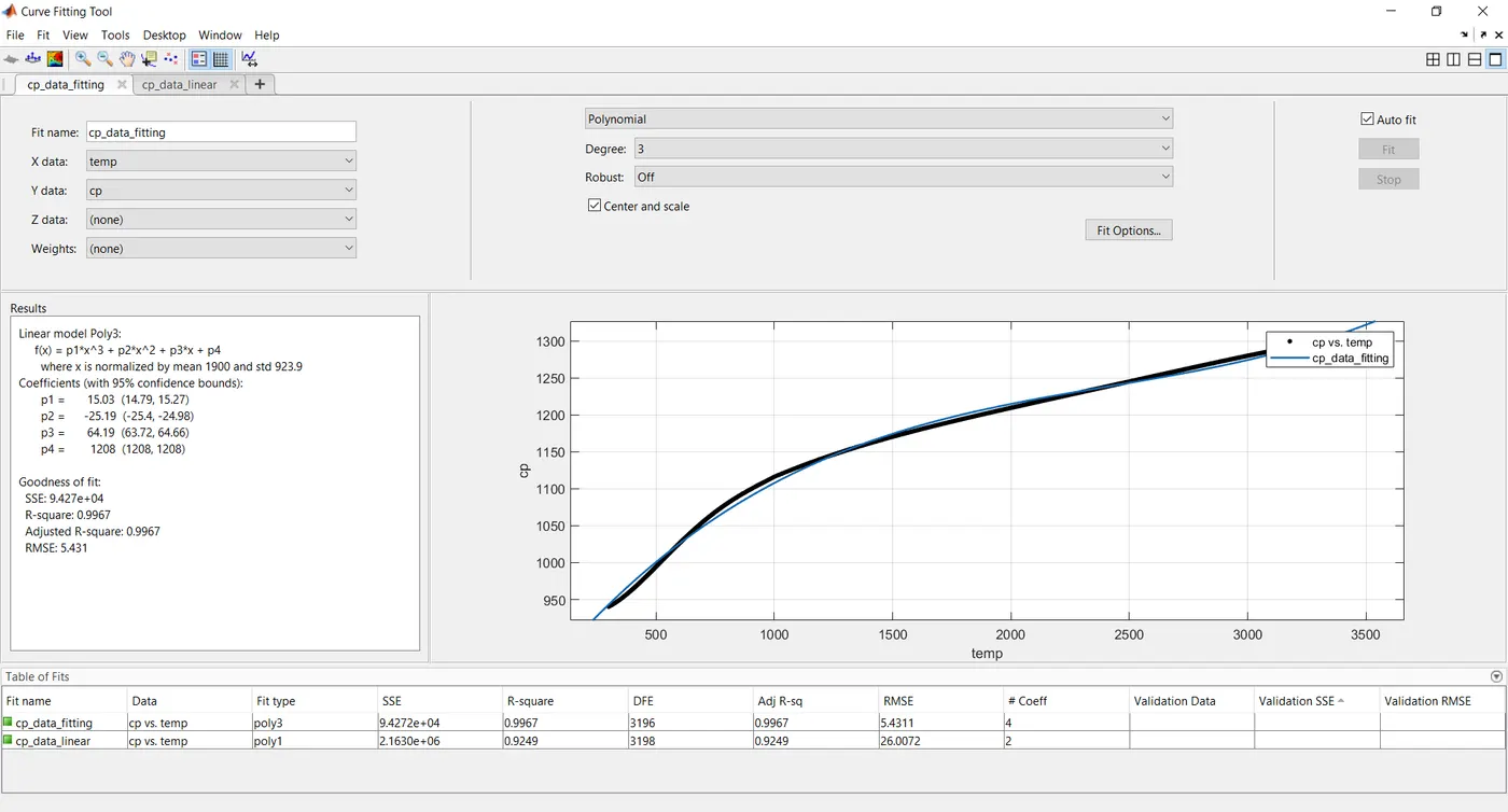
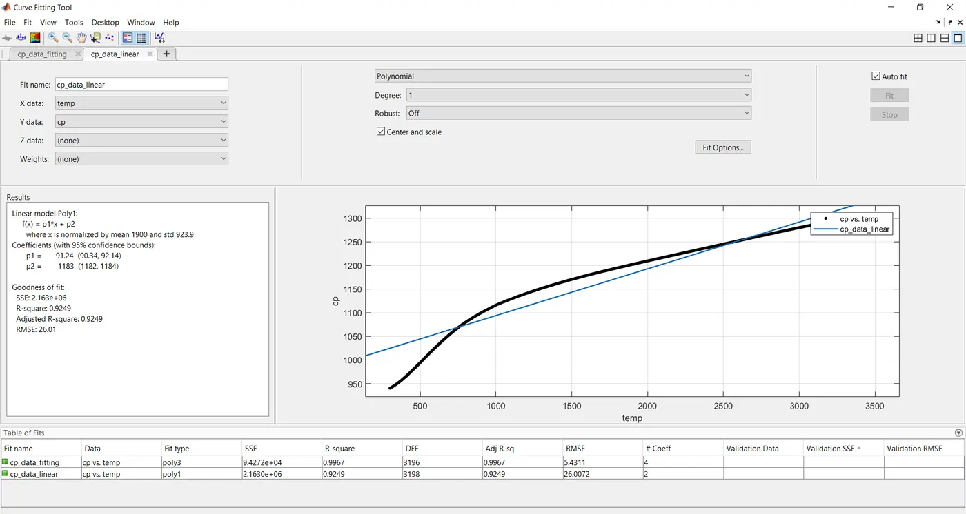
- Performed cubic fit and linear fit in Curve Fitting TOOL and compared it to previously created fitting algorithm and found it to be nearly same, implying the custom fitting algorithm is correct.
Conclusion-
From the understanding of this Mini-project we can say a perfect fit can be obtained by several methods like
- Interpolation by which errors can reduced to zero.
- Centering and Scaling can be done to fit a particular order of polynomial.
In a simple way, the basic idea is to minimise the residual errors to get perfect fit. To obtain the best fit we increase the degree of the polynomial or also we can use split wise regression technique.A cubic fit can be improved by using
- Centering & Scaling method
- By diving temperature into different ranges and using split wise regression technique.